Interfacial Heat Transfer Coefficient Calibration under Injection Cavity Pressure Curves
Calibrating interfacial heat transfer against cavity pressure curves replaces guess-work with exact pressure-dependent thermal conductance functions.
Boundary
Heat extraction across the steel-polymer threshold governs part crystallization, cycle timing, and structural warpage in injection moulding. Thermal conductance at this surface is not constant. The interfacial heat transfer coefficient fluctuates by an order of magnitude between initial cavity filling and final part ejection, driven primarily by local contact pressure.
During initial melt entry and high-pressure packing, molten polymer establishes intimate microscopic contact with the tool wall, flattening surface roughness asperities and forcing trapped air out of microscopic valleys. Thermal conductance reaches peak values between 2500 W/m²K and 6000 W/m²K under full holding pressure. As the gate freezes and volumetric shrinkage accelerates, cavity pressure decays rapidly.
Lower contact pressure allows microscopic detachment, reducing thermal transmission before a macro-scale gap develops. When local pressure drops toward ambient, physical detachment creates an insulating air gap, plunging the heat transfer coefficient to values between 100 W/m²K and 300 W/m²K.
Melt State and Interfacial Resistance Transitions
Conduction across the tool wall responds directly to the mechanical state of the solidifying polymer skin. The primary resistance to heat flow shifts through three distinct regimes across a standard injection cycle. The initial filling phase establishes hydrodynamic contact under low contact pressure, yielding moderate thermal transmission rates.
The holding pressure phase deforms the cooling solid skin into micro-topographical tool features, maximizing effective contact area. The cooling phase induces thermal contraction that eventually overcomes cavity pressure, causing boundary separation. CAE simulations assuming a static interfacial conductance value fail to capture early-stage skin formation and late-stage core cooling rates.
This mismatch distorts predicted volumetric shrinkage and residual stress profiles.
Quantifying the thermal conductance function requires synchronized measurement of transient wall temperature and local cavity pressure. Thermocouples embedded flush with the cavity surface record steep thermal transients, while piezoelectric transducers capture pressure decay curves. Processing these twin signals through inverse numerical methods extracts the dynamic interfacial conductivity as an explicit function of cavity pressure and cooling time.
Local contact pressure during the packing phase increases effective interface conductivity up to twenty times above the air-gap decoupled baseline.
The relationship between cavity pressure Pcavity and the heat transfer coefficient heff appears in empirical formulations as a non-linear power-law function. At elevated pressure, solid-to-solid contact dominates thermal transport. At zero relative cavity pressure, radiation and gaseous conduction through thin air pockets take over.
Tool steel polish, surface coatings, and thermal diffusivity further alter the absolute magnitude of heat flux across this interface.
Pressure-Thermal Coupling Mechanics
Pressure controls thermal contact resistance by modifying the effective real contact area between the semi-solid polymer shell and the steel wall. Machine pressure pushes micro-asperities into plastic deformation, forcing polymer chains into intimate contact with metallic grains. Higher packing pressures yield thicker, more rapidly developed solid frozen layers, altering the internal temperature gradient of the part wall.
When cavity pressure drops below a critical threshold, thermal contraction pulls the solidifying skin inward, creating a vacuum or low-pressure air boundary.
| Process Phase | Cavity Pressure Range (bar) | Interfacial Contact Mode | Typical Conductance (W/m²K) |
|---|---|---|---|
| Filling | 50 – 250 | Dynamic Fluid Shear Contact | 1000 – 2000 |
| Packing Peak | 300 – 1200 | Deformed Asperities Static Contact | 3500 – 6000 |
| Pressure Decay | 20 – 300 | Partial Surface Detachment | 500 – 1500 |
| Cooling Post-Gate Freeze | 0 – 20 | Insulated Air Gap Separation | 100 – 300 |
Disregarding the pressure dependence of interfacial conductance leads to severe overestimation of cooling efficiency during the late cycle. Numerical solvers that apply an uncalibrated fixed coefficient generate part temperature profiles that predict premature ejection readiness. Tools built against these flawed assumptions deliver parts with unpredicted core temperatures, resulting in severe post-moulding warpage, unexpected sink marks, and extended cooling cycle times on the shop floor.
Gap
Microscopic void formation at the tool interface creates a thermal barrier that dominates cooling dynamics once local pressure falls below material yield limits. As molten polymer cools, its volumetric specific mass decreases in accordance with its pressure-volume-temperature properties. High cavity pressure delays physical separation by forcing the elastic polymer skin to deform outward against the contracting interior core.
The moment internal pressure drops below the force necessary to maintain outer shell deformation, microscopic air pockets merge into a continuous thermal separation layer.
Asperity Deformation and Surface Roughness Dynamics
Tool steel roughness directly governs the contact area achieved under specific cavity pressure levels. EDM finishes create sharp micro-peaks that pierce the polymer skin, establishing localized high-conduction pathways while trapping air in deep valley pockets. Polished optical steel surfaces yield uniform contact areas at lower pressures, yet suffer drastic conductance losses the moment thermal contraction breaks surface contact.
Tool surface roughness metrics Ra and Rz define the theoretical maximum heat transfer coefficient achievable at complete material yield.
Pressuring the melt compresses trapped micro-air pockets inside steel valleys, raising the conductive property of the trapped gas medium. When cavity pressure decays during gate freeze, these compressed air micro-pockets expand, forcing the soft polymer skin off the tool wall before macro-scale thermal contraction occurs. This micro-detachment phase initiates the drop in interfacial thermal conductance long before standard linear displacement sensors detect physical part shrinkage.

Thermal Resistance Stacking across Interface
Total heat flow per unit area across the tool interface follows a series thermal resistance model containing three distinct components:
- Bulk Polymer Shell Resistance governs conduction from the molten inner core through the solidifying skin layer, governed by intrinsic material conductivity.
- Interfacial Contact Resistance acts at the steel-polymer surface junction, varying continuously as cavity pressure deforms skin micro-asperities.
- Tool Steel Wall Resistance manages heat transport away from the cavity surface into internal cooling lines, governed by tool steel grade selection.
Part detachment occurs earlier in thick wall sections than in thin ribs due to higher total volumetric shrinkage potential. High cooling rates solidify outer polymer layers rapidly, building bending stiffness in the skin that resists remaining cavity pressure. Thick parts develop high internal tensile stresses that pull the skin away from tool steel walls well before the cavity reaches ambient pressure.
Interfacial thermal contact resistance dominates total wall thermal resistance during the initial twenty percent of the cooling time.
The air gap thickens dynamically as cooling continues, plateauing when the core polymer drops below its glass transition temperature or crystallization end-point. Beyond this threshold, part dimensions stabilize inside the cavity, establishing a final air gap clearance dictated by shrinkage thermodynamics and part restraint constraints imposed by core pins. A small rule of thumb governs this boundary stage: higher cavity packing pressure delays gap formation but cannot prevent it once volumetric shrinkage exceeds elastic strain limits.
Sensor
Capturing high-resolution pressure decay profiles requires dynamic instrumentation capable of operating inside high-temperature, high-pressure tool environments. Piezoelectric quartz pressure sensors installed directly behind cavity pins deliver high frequency response without introducing surface thermal anomalies. These sensors capture pressure signals at acquisition frequencies of 1 kHz or greater, resolving minute pressure steps during gate freeze and skin detachment events.
Simultaneously, coaxial fast-response thermocouples mounted flush with the cavity wall record surface thermal spikes and subsequent exponential cooling decay curves.
Instrumentation Setup and Spatial Sensor Placement
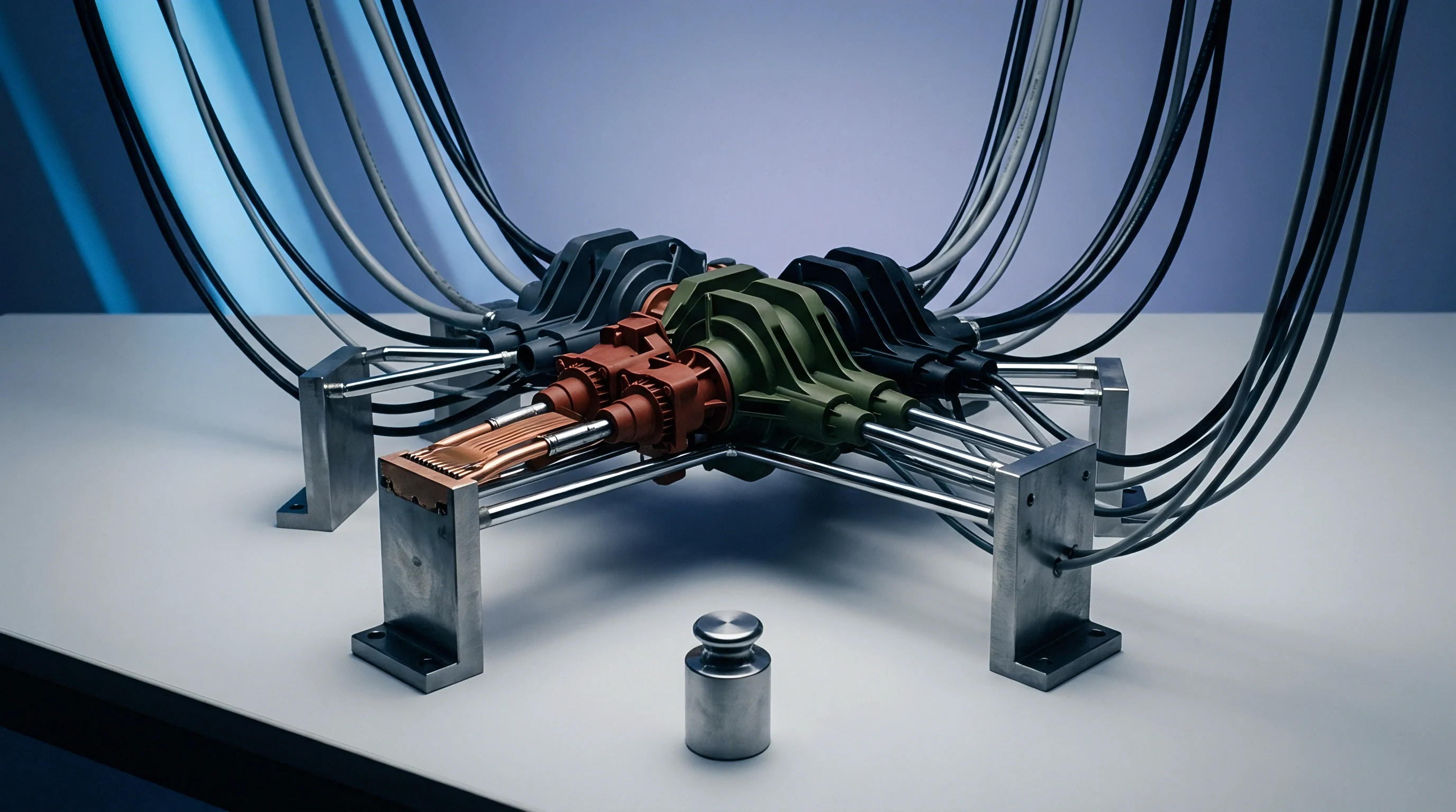
Selecting measurement locations requires placing transducer pairs along the fill path to record spatial variations in contact pressure and cooling history. Ideal locations include points near the gate, mid-cavity regions, and the end of fill. Near-gate transducers capture prolonged high-pressure regimes, whereas end-of-fill sensors record early pressure drop-off and premature air gap initiation.
Indirect pressure sensors mounted behind ejector pins introduce mechanical compliance and friction delays that smooth out sharp pressure transitions. Direct surface-mount quartz sensors eliminate pin friction, yielding accurate cavity pressure derivatives needed for precise thermal calibration. Combining a fast-response E-type surface thermocouple with a direct quartz pressure sensor inside a single combined housing minimizes spatial distance, ensuring tight temporal synchronization between thermal and pressure signals.
Signal Processing and Noise Suppression
Raw cavity pressure profiles carry mechanical vibrations from press hydraulics, screw recovery, and tool platen deflections. Applying digital Butterworth low-pass filters removes high-frequency electrical noise while preserving the rapid pressure drop-off derivative during gate sealing. Thermal signals from surface thermocouples undergo numerical inverse filtering to reconstruct true surface heat flux, accounting for thermocouple junction depth variations and localized thermal mass disturbances.
| Measurement Variable | Sensor Technology Type | Sampling Rate Required | Primary Error Mechanism |
|---|---|---|---|
| Cavity Pressure | Direct Piezoelectric Quartz | 1000 Hz | Charge amplifier drift over long cycles |
| Cavity Pressure | Indirect Ejector Pin Load Cell | 500 Hz | Pin friction and mechanical clearance hysteresis |
| Tool Surface Temp | Coaxial Flush Thermocouple | 1000 Hz | Thermal mass offset of sensor tip junction |
| Part Wall Temp | Infrared Fiber-Optic Sensor | 200 Hz | Uncertain melt emissivity during phase change |
Data acquisition hardware must sample pressure and thermal channels simultaneously on a unified clock board to avoid temporal skew. A temporal offset of even 10 milliseconds between the pressure decay slope and the thermal response curve distorts the calculated heat transfer coefficient function, falsely shifting the calculated contact resistance onset timing.
When discrepancies occur between physical parts and simulation models, tooling suppliers frequently claim that standard datasheet thermal constants represent tool behavior across all pressure ranges. This assertion ignores the physical reality of pressure-dependent contact resistance observed on active production tooling.
Solver
Determining the heat transfer coefficient from measured pressure and thermal curves represents a classical Inverse Heat Conduction Problem. Direct heat conduction calculations predict temperature fields from known boundary conditions. Inverse methods work backward, calculating unknown surface heat flux and thermal contact resistance from transient internal temperature data.
Mathematical algorithms iterate numerical thermal models until calculated boundary temperatures match experimental thermocouple traces within tight convergence limits.
Inverse Heat Conduction Mathematical Formulations
The one-dimensional transient heat conduction equation within the tool steel domain provides the core numerical formulation for thermal inversion:
ρ cp fracpartial Tpartial t = fracpartialpartial x left( k fracpartial Tpartial x right)
Here, ρ represents steel density, cp denotes specific heat capacity, and k is thermal conductivity. The boundary condition at the cavity interface x = 0 directly incorporates the dynamic interfacial heat transfer coefficient h(P, t) and the transient polymer skin temperature Tp(t) relative to the steel surface temperature Ts(t):
q”(t) = -k left. fracpartial Tpartial x right|x=0 = h(P, t) · left( Tp(t) – Ts(t) right)
Inverse solvers apply optimization algorithms such as the Levenberg-Marquardt method or Conjugate Gradient Method to minimize an objective function J. This function calculates the sum of squared errors between experimental temperature values Yi and model-predicted temperatures Ti across discrete time steps:
J(h) = sumi=1N left( Yi – Ti(h) right)2
Numerical regularization techniques, including Tikhonov regularization, prevent instability and noise amplification during mathematical differentiation of experimental thermal signals.
- Signal Acquisition and Conditioning imports raw cavity pressure and surface temperature traces, removing high-frequency electrical interference through digital filtering algorithms.
- Forward Thermal Solver Initialization sets baseline material properties, tool mesh configurations, and initial melt temperature distribution estimates.
- Iterative Parameter Parameterization adjusts polynomial or piecewise linear coefficients defining the h(P) function based on objective function gradients.
- Residual Convergence Check evaluates calculated surface thermal matches against predefined tolerance thresholds to complete the parameter calibration loop.
What Limits Single Parameter Pressure Curve Thermal Calibration Accuracy?
Calibrating h(P) strictly as a single-variable function of cavity pressure introduces errors when thermal contraction occurs independently of local pressure decay. In complex part geometries with severe wall thickness steps or constrained core pins, shear stresses and differential volumetric shrinkage break surface contact while cavity pressure remains elevated elsewhere in the runner system. Advanced inverse solvers address this limitation by formulating heat transfer coefficients as dual-variable surfaces h(P, vshrinkage), coupling local pressure traces directly to local volumetric strain calculations derived from state equations.
Iterative optimization runs until the residual sum of squares between measured and simulated surface temperatures drops below 10-6. Solvers operating on incomplete pressure traces produce non-unique numerical solutions, where multiple different h(P) curves generate identical surface temperature traces. Enforcing monotonicity constraints on the inverse mathematical solver prevents non-physical oscillations in calculated thermal transmission values.
Uncertainty remains regarding whether local shear deformation during the filling phase temporarily raises interfacial thermal conductance above static pressure limits. Resolving this requires non-invasive sub-millisecond optical measurements of melt contact physics directly at the steel surface during fill.
Polymers
Polymer morphology fundamentally dictates how interfacial contact thermal conductance responds to cavity pressure history. Semicrystalline resins undergo sharp density shifts during crystallization, triggering sudden micro-detachment events that sharply lower heat transfer rates. Amorphous polymers exhibit gradual, predictable volume changes across their glass transition range, producing smooth conductance decay curves that track cavity pressure loss linearly.
Semicrystalline versus Amorphous Detachment Physics
Polypropylene, polyamide, and polybutylene terephthalate undergo significant volumetric contraction when polymer chains align into ordered crystalline lattices. This phase transition releases latent heat of crystallization while simultaneously accelerating spatial volume reduction. The resulting rapid shrinkage forces early skin separation from cavity walls, causing an abrupt drop in heat conductance even when holding pressure remains active at the machine nozzle.
Amorphous resins like polycarbonate, acrylonitrile butadiene styrene, and polysulfone maintain an amorphous molecular matrix during cooling. Volumetric contraction follows smooth pressure-volume-temperature curves governed by glass transition boundaries. Consequently, these materials maintain intimate surface contact longer under decaying cavity pressure, exhibiting extended high-conductance regimes compared to semicrystalline compounds.
Reinforcing fillers alter interfacial heat transfer dynamics through two concurrent physical mechanisms. Inorganic fillers like glass fibers and mineral additives raise bulk polymer thermal conductivity, accelerating heat transport from the interior core to the outer skin shell. Simultaneously, non-yielding glass fibers stiffen the frozen outer layer, increasing resistance to elastic deformation under internal pressure.
This added structural stiffness causes skin separation at higher residual cavity pressures, narrowing the time window during which peak interfacial thermal conductance applies.
| Polymer Family | Morphology Type | Volumetric Shrinkage Range (%) | Peak Pressure Conductance (W/m²K) | Detachment Conductance (W/m²K) |
|---|---|---|---|---|
| Polypropylene (PP) | Unfilled Semicrystalline | 1.5 – 2.2 | 3000 – 4500 | 120 – 180 |
| Polyamide 66 (PA66 GF30) | 30% Glass Semicrystalline | 0.4 – 0.8 | 4500 – 6500 | 200 – 350 |
| Polycarbonate (PC) | Unfilled Amorphous | 0.5 – 0.7 | 2500 – 3800 | 150 – 220 |
| ABS / PC Blend | Unfilled Amorphous Alloy | 0.4 – 0.6 | 2800 – 4000 | 140 – 200 |
Processing Window Effects on Interface Thermal Dynamics
Modifying melt and tool temperature parameters changes the effective boundary conductances calculated from cavity pressure curves. Higher tool steel temperatures delay outer skin freezing, allowing cavity pressure to force soft polymer chains deeper into steel surface micro-grooves. This process increases effective contact area and raises peak interfacial heat transfer coefficient values.
Lower melt temperatures increase initial resin viscosity during filling, creating a thicker, stiffer frozen skin layer during early injection. This rigid skin resists outer boundary deformation under holding pressure, preventing optimal microscopic contact with cavity walls and reducing achievable peak heat transfer coefficients across all pressure regimes.
High holding pressure extends the time window of maximum contact conductance, forcing heat out of the part rapidly during early cooling steps. Once gate freeze occurs, cavity pressure drops to zero as volume loss continues unmanaged within the runner system. Beyond this transition point, heat transfer across the interface depends entirely on residual air gap thermal conductivity, rendering machine pressure adjustments ineffective.

Audit
Calibrating heat transfer coefficients against cavity pressure curves provides essential engineering data required to validate tooling designs prior to mass production commitments. Standard CAE simulation templates rely on default, static heat transfer values that fail to capture pressure-dependent cooling dynamics. Integrating pressure-calibrated thermal functions into simulation workflows eliminates spatial cooling rate errors, allowing precise prediction of warpage, sink marks, and true minimum required cycle times.
CAE Calibration Validation Protocols
Validating simulation accuracy requires comparing calculated cavity pressure decay traces directly against physical transducer data gathered during tool trials. A misaligned pressure decay slope indicates incorrect interfacial thermal conductance functions within the simulation setup, leading to inaccurate part deformation predictions.
Simulations using static heat transfer coefficients often underestimate cooling times for thick-walled components by fifteen to thirty percent. Applying pressure-calibrated conductance functions aligns predicted part wall temperature profiles with actual physical cooling times recorded during press bring-up trials. This alignment ensures accurate cycle time estimation during quote phases, preventing commercial losses driven by unexpected cooling extensions on production floors.
Precise thermal boundary calibration allows accurate calculation of residual stress accumulation during the transition from packing to air gap formation. Differential cooling across opposing cavity faces drives part warpage. Applying localized, pressure-calibrated heat transfer functions enables tool designers to optimize cooling line placements, adjusting localized steel temperatures to counteract thermal imbalance before cutting metal.
Discrepancies between predicted and actual warpage vectors drop below eight percent when pressure-dependent heat transfer functions replace static simulation values.
Tooling sign-off procedures specify dimensional tolerance verification under standardized environmental conditions according to DIN 16742 guidelines. Incorporating pressure-calibrated thermal simulation parameters into tool design phase gates ensures parts achieve specified tolerance grades without requiring costly post-machining cooling circuit modifications.
Commercial Risk Allocation and Specification Sign-Off
Tooling purchase agreements must explicitly define the thermal boundary conditions and simulation setup parameters used to validate part ejection readiness and cycle time guarantees. Relying on default software properties creates commercial exposure when tools fail to meet promised cycle times during factory acceptance testing.
A standard contract specification clause reads: Tooling cycle time acceptance testing requires cavity pressure transducers to confirm that local interfacial thermal conductance values match verified CAE input tables within a five percent margin before final steel sign-off. Incorporating this language shifts financial risk from the part buyer to the toolmaker, enforcing rigorous scientific simulation practices before steel cutting begins.