Multiphysics Solver Calibration for Cavity Pressure Dependent Thermal Conductance
Calibrate solver thermal conductance against in-tool pressure and temperature telemetry to prevent costly mold re-cutting loops and secure tight tolerances.
Contact
The physical mechanism linking thermal energy transfer to mechanical force at the polymer-steel boundary dictates heat extraction speed during injection moulding. Polymer melt entering a steel mold cavity encounters microscopic surface irregularities on the cavity wall. As high injection pressure forces liquid resin against tool steel, the melt deforms into microscopic asperities, air is displaced from interfacial valleys, and real contact surface area approaches physical limits.
High local packing pressure maximizes thermal contact conductance across the interface, elevating thermal dissipation rates. When the polymer cools and solidifies, volumetric thermal contraction initiates, cavity pressure decays, and mechanical strain lifts the cooling skin away from tool steel. This detachment opens an insulating air gap that reduces local thermal transport by orders of magnitude.
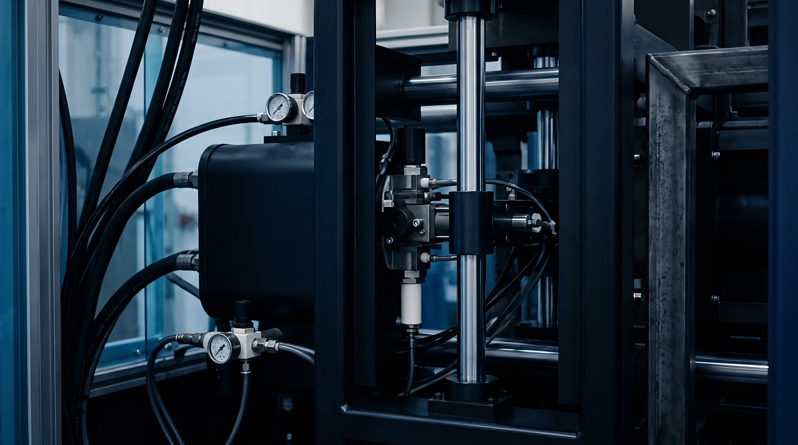
Interfacial Heat Boundary Behavior across Injection Phases
Polymer melt entering a steel mold cavity encounters a rapid transient thermal state. During initial filling, high shear rates and velocity vectors keep liquid polymer pressed against polished or textured tool steel. Thermal contact conductance, expressed as an interfacial heat transfer coefficient in units of watts per square meter-kelvin, reaches baseline liquid values ranging from six hundred to one thousand watts per square meter-kelvin.
Once the cavity fills and the machine transitions to velocity-to-pressure switchover, packing pressure escalates local cavity pressure to levels between twenty megapascals and one hundred twenty megapascals. Surface roughness governs initial boundary contact. Pressure forces melt into micro asperities.
This peak pressure phase compresses micro-scale gas pockets trapped in cavity wall surface roughness profiles. Under maximum cavity pressure, thermal contact conductance reaches peak values, exceeding two thousand five hundred watts per square meter-kelvin for semi-crystalline polymers such as polypropylene and polyoxymethylene. Increased chain packing density in semi-crystalline resins accelerates heat removal, elevating local thermal diffusivity.
Amorphous polymers like polycarbonate and ABS exhibit lower peak thermal conductance values under identical pressure conditions due to lower inherent thermal conductivity and higher melt elasticity. As cooling continues, gate freeze-off halts pressure transmission from the injection unit. The thermal boundary layer collapses rapidly.
An increase in packing pressure from 20 MPa to 60 MPa elevates interfacial thermal conductance from 800 W/m²K to 2200 W/m²K in semi-crystalline resins.
Cavity pressure decays as the solidifying core shrinks. When local cavity pressure drops below a critical mechanical threshold, elastic recovery of tool steel and volumetric thermal shrinkage of the polymer polymer skin decouple the interface. An air gap opens, introducing an insulating barrier with thermal conductivity near zero point zero two six watts per meter-kelvin.
Air gaps create severe thermal resistance. Local interfacial heat transfer coefficients plunge below two hundred watts per square meter-kelvin. Standard multiphysics solvers utilizing static, temperature-independent heat transfer coefficients fail to capture this non-linear transition, miscalculating total cooling time and downstream thermal warpage vectors.

Mathematical Formulation of Pressure Dependent Conductance Curves
Numerical solvers represent boundary thermal transport using non-linear mathematical expressions that link heat transfer coefficients directly to local cavity pressure. A piecewise linear or exponential decay formulation models the transition between intimate tool contact, pressure-dependent contact, and open-gap detachment. Equation models express the interfacial conductance as a function of instantaneous pressure:
The formulation incorporates three distinct operational domains: an open-gap baseline conductance value, a pressure-sensitivity coefficient governing early packing contact, and a asymptotic maximum conductance corresponding to complete surface compliance. In solver implementations, local pressure calculated at boundary nodes determines the instantaneous heat flux entering the mold cooling mesh. Without proper empirical calibration of these mathematical parameters, numerical solvers miscalculate core thermal gradients, misjudging the freeze-off point of narrow wall sections and ribbed structural features.
| Processing Phase | Cavity Pressure Range (MPa) | Amorphous Resins (W/m²K) | Semi-Crystalline Resins (W/m²K) | Interfacial Contact State |
|---|---|---|---|---|
| Filling Phase | 2.0 – 15.0 | 400 – 750 | 500 – 900 | Hydrodynamic Contact |
| Packing Peak | 30.0 – 100.0 | 1200 – 1800 | 1800 – 3200 | Asperity Deformation |
| Cooling Decay | 5.0 – 25.0 | 500 – 900 | 650 – 1200 | Partial Pressure Contact |
| Part Detachment | 0.0 – 2.0 | 80 – 220 | 100 – 250 | Insulating Air Gap |
Inaccurate boundary conductance modeling generates cumulative errors throughout the entire multiphysics simulation workflow. Uncalibrated solvers underpredict final warpage. Miscalculated cooling rates alter predicted volumetric shrinkage distributions, throwing off dimension calculations specified under DIN 16742 tolerance classes.
When solver boundary conditions overestimate heat extraction during packing, predicted part cycle times come out artificially short, leading toolmakers to build cooling circuits that underperform on production presses.
- Skin Thickness Miscalculation occurs when overestimated conductance during early cooling accelerates predicted surface freezing, masking flow-front instabilities and void risk.
- Differential Shrinkage Errors arise from uniform heat transfer assumptions across core and cavity sides, causing inaccurate predictions of part bowing and angular distortion.
- Gate Freeze Timing Flaws result from misjudging thermal transport during packing, causing solvers to miscalculate the mass entering the cavity during hold pressure.
- Ejection Force Underestimation develops when solver temperature outputs understate final part core temperature, leading to unexpected vacuum creation and rib sticking during press opening.
Failure to calibrate pressure-dependent thermal conductance functions causes finite element simulation packages to generate misleading thermal histories, resulting in tool modifications that cost thousands of dollars per iteration cycle.
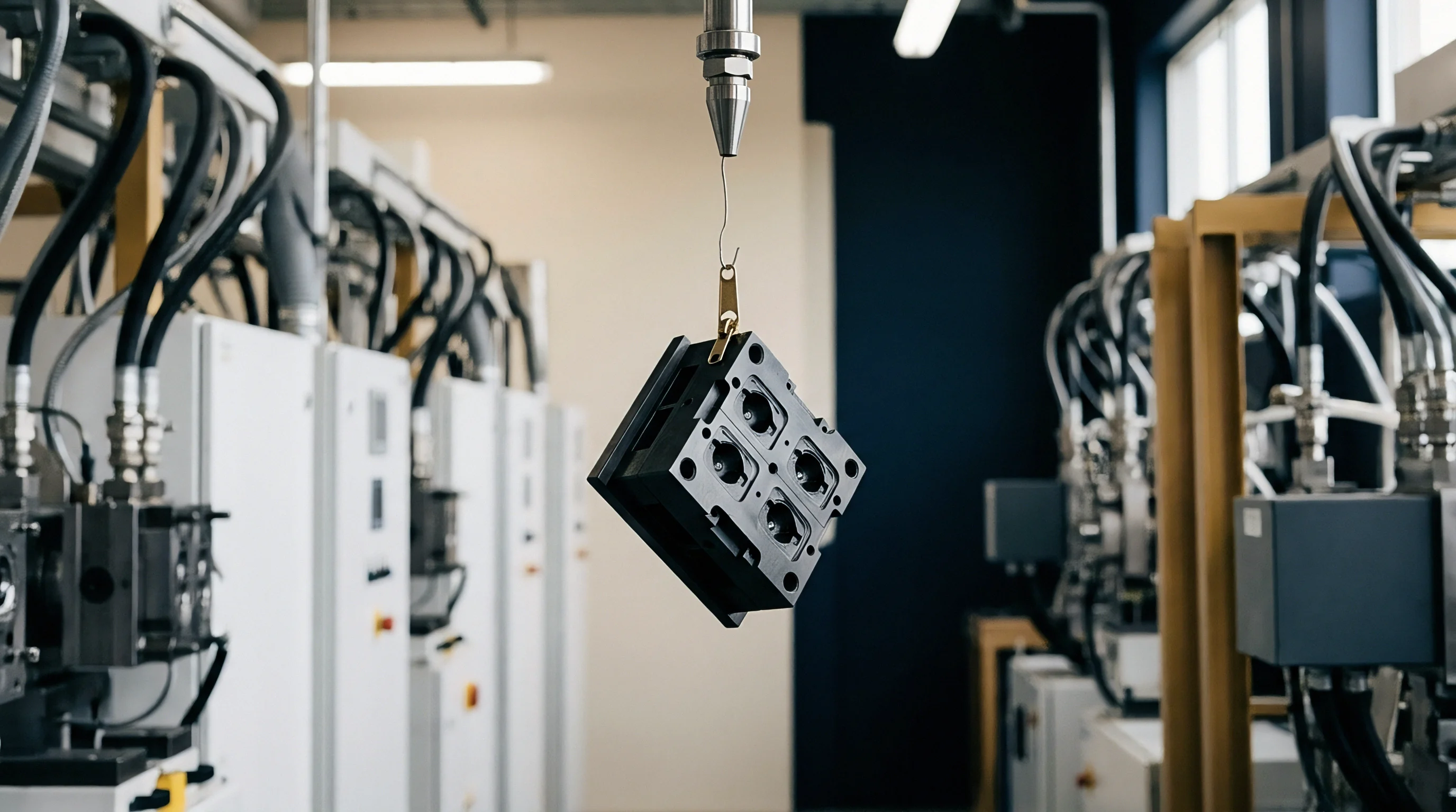
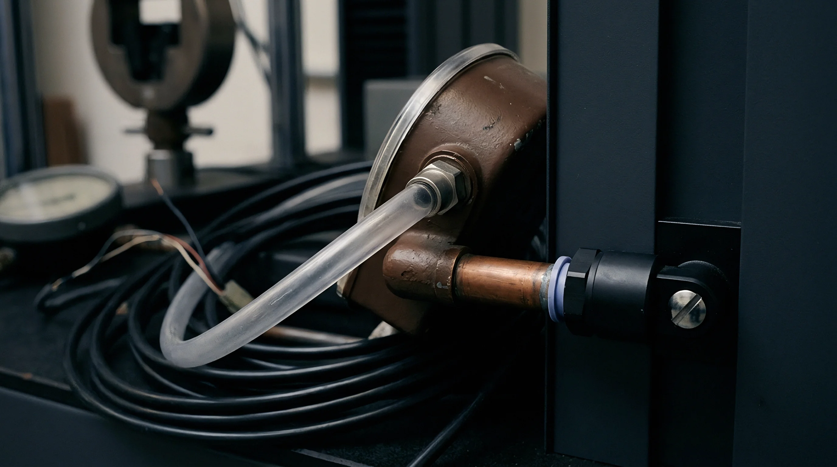
Telemetry
Real-time empirical datasets provide the baseline inputs required to tune multiphysics heat transfer boundary conditions. Capturing precise thermal and mechanical events inside a hardened steel injection mold demands specialized sensor hardware flush-mounted directly at the mold-cavity interface. Single-point cavity temperature readings from standard thermocouples lack the spatial resolution and temporal response speed necessary to resolve steep thermal gradients that develop within milliseconds of melt contact.
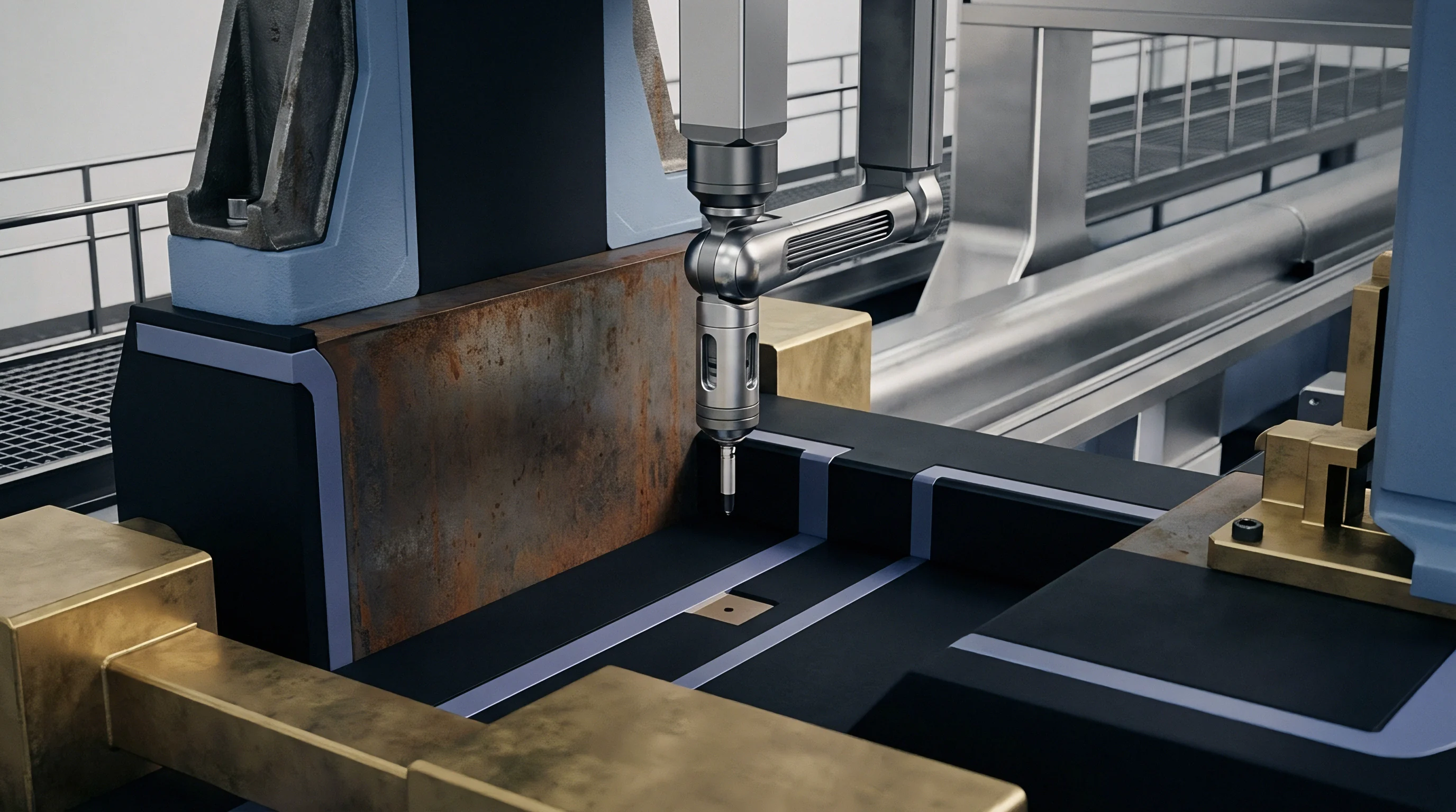
In-Tool Sensor Integration for Transient Heat Flux Measurement
Hardware embedded directly inside mold steel captures simultaneous pressure traces and rapid surface temperature shifts. Combined piezoelectric pressure and fast-response surface thermocouple sensors provide dual-channel telemetry from a single cavity penetration hole. Sensor design incorporates a piezoelectric quartz element surrounding a thin-film thermocouple junction composed of iron and constantan or type K alloys.
The surface thermocouple junction lies within micrometers of the sensor front face, yielding thermal response times below two milliseconds. Sensor alignment determines signal fidelity.
Positioning transducer locations along the melt flow length ensures accurate capturing of pressure decay dynamics. Primary sensors sit adjacent to the main feed gate, where peak packing pressure occurs. Secondary sensors occupy mid-cavity wall regions, while tertiary transducers sit near the end of fill, where cavity pressure drops rapidly and air entrapment or thermal hesitation occurs.
Piezoelectric elements record sharp pressure rises. Fast-response sensor installations require absolute flush mounting relative to cavity steel surfaces. Sensor protrusion into the melt stream induces local shear heating, corrupting thermal boundary data.
Sensor recession creates melt dead zones that delay thermal response and create false pressure decay signatures.
Adherence to ISO 294-1 mold temperature sensor positioning rules guarantees thermal boundary conditions match solver mesh nodes within two tenths of a millimeter.
Sensor wiring routes through machined wire slots in backer plates, terminating at multi-channel charge amplifiers and data acquisition interfaces. Signal transmission requires high-insulation cables protected from environmental humidity and oil contamination to maintain gigohm-level insulation resistance on piezoelectric outputs. Thermocouple response times dictate sampling speed.

Transducer Signal Conditioning and Sampling Synchronization
High-speed digital conversion transforms analog millivolt signals and picocoulomb charge outputs into synchronized time-series data arrays. Data acquisition cards process pressure and temperature channels at sampling frequencies equal to or exceeding one kilohertz per channel. High-frequency sampling captures the exact instant of melt contact, peak pressure attainment, and pressure drop during gate freeze.
Thermocouple millivolt outputs pass through low-noise cold-junction compensation circuitry, while piezoelectric charge signals run through precision charge amplifiers set to matched measuring ranges. Noise filtering prevents solver divergence.
| Parameter | Combined Piezo-Thermocouple | Piezoresistive Strain Sensor | Eroded Surface Thermocouple |
|---|---|---|---|
| Pressure Range (MPa) | 0 – 250 | 0 – 200 | N/A (Temperature Only) |
| Temperature Range (°C) | 0 – 400 | 0 – 200 | 0 – 450 |
| Thermal Response Time | < 2.0 ms | < 15.0 ms | < 0.5 ms |
| Pressure Sensor Accuracy | ± 0.5% Full Scale | ± 1.0% Full Scale | N/A |
| Mounting Diameter (mm) | 4.0 – 6.0 | 2.5 – 4.0 | 1.0 – 2.5 |
Signal synchronization across independent channels remains essential for accurate parameter identification. Time stamps for pressure rise and thermal jump points must align within one millisecond. Thermal contact conductance calculations derive directly from the transient heat flux vector, computed using one-dimensional inverse conduction equations applied to the steel boundary layer temperature curve.
Synchronized pressure traces provide the independent variable axis, mapping calculated instantaneous conductance values against cavity pressure.
- Sensor Installation Depth demands precision machining to keep transducer faces flush within zero point zero one millimeters of cavity steel.
- Amplifier Sampling Frequency must operate at one kilohertz minimum to catch high-speed pressure peaks during switchover.
- Thermal Drift Compensation adjusts sensor zero balances between molding cycles to prevent baseline shift errors.
- Spatial Transducer Spacing assigns at least three dual-sensor locations along the flow channel length to map pressure gradients accurately.
Tooling vendors often claim that factory-default solver conductance values eliminate the need for in-tool sensor instrumentation, asserting that standard polymer thermal diffusivity tables cover real molding conditions without custom press trials.
Inversion
Optimizing thermal parameters requires fitting calculated profiles from numerical simulation models to measured temperature curves acquired during tool trials. Direct measurement of thermal contact conductance at the polymer-steel interface proves extremely difficult due to the thinness of the boundary region and high transient rates. Inverse Heat Conduction Problem algorithms resolve this challenge by using internal steel temperature histories to calculate heat flux and interfacial boundary conductance backwards in time.
When Does Solved Heat Flux Diverge from Measured Polymer Cooling?
Discrepancies arise primarily during the transition from high-pressure packing to cooling pressure decay. Decoupled solver runs that treat thermal conductance as a static step function miscalculate heat loss during early cooling. At the instant of melt contact, measured steel surface temperature jumps rapidly, reaching a peak value that reflects the initial contact resistance.
As cavity pressure rises, heat flux increases sharp, driven by expanding micro-scale contact area between resin and steel. Convergence requires tight residual bounds.
When packing pressure drops, measured steel temperature curves exhibit an inflection point where the cooling rate slows down abruptly. Standard solver models using constant heat transfer coefficients continue predicting rapid thermal discharge, creating a divergence gap between virtual and experimental temperature profiles. This divergence becomes severe in thick-walled section geometry where internal thermal mass maintains core melt temperature while the frozen outer skin pulls away from mold steel under thermal strain.
Iterative loops update boundary coefficients.
Non Linear Inverse Heat Conduction Parameter Estimation
Mathematical algorithms solve boundary optimization loops through iterative parameter modification. The objective function minimizes the sum of squared differences between calculated finite element node temperatures and experimental surface thermocouple datasets over the full molding cycle time:
Levenberg-Marquardt optimization routines adjust the coefficient matrix governing the pressure-dependent conductance function until calculated thermal curves converge onto empirical thermocouple tracks. The algorithm calculates sensitivity coefficients, representing the partial derivative of local boundary temperature with respect to each conductance model parameter. High sensitivity coefficients indicate parameters that exert strong control over solver output, ensuring stable convergence during parameter estimation runs.
Calibrating thermal conductance against static pressure traces fails when melt solidification precedes maximum cavity packing.
A representative optimization case demonstrates the impact of proper inverse calibration on a three-millimeter polyoxymethylene housing component. Initial uncalibrated simulation runs using default solver coefficients predicted a total cycle time of sixteen point two seconds, with an end-of-cooling surface temperature of fifty-eight degrees Celsius. empirical press trials using flush-mounted sensors revealed real part ejection temperatures reaching seventy-four degrees Celsius, causing part warpage exceeding component drawing tolerances.
1. Define initial parameter bounds for maximum packing conductance, residual gap conductance, and exponential pressure decay coefficients based on resin capillary rheology.
2. Map experimental pressure-time histories into boundary conditions across solver boundary mesh elements.
3. Run forward multiphysics thermal solver passes to output transient temperature fields at virtual sensor node coordinates.
4. Compute gradient matrices for local temperature residuals with respect to conductance parameters.
5. Update pressure-dependent conductance coefficients using damped non-linear optimization iterations until root-mean-square error falls below target thresholds.
Executing the inverse calibration procedure generated calibrated parameters: a maximum packing conductance of two thousand eight hundred watts per square meter-kelvin, an open-gap baseline of one hundred twenty watts per square meter-kelvin, and a pressure decay sensitivity coefficient of zero point zero four five per megapascal. Updating solver material databases with these calibrated values aligned simulated surface cooling curves within one point five degrees Celsius of experimental sensor data. Predicted volumetric shrinkage matched actual part measurements across three independent production lots, eliminating secondary tooling modifications.
Parameter calibration routines perform accurately only when transient sensor data is gathered under thermal steady-state mold conditions after at least thirty continuous press cycles.
Coupling
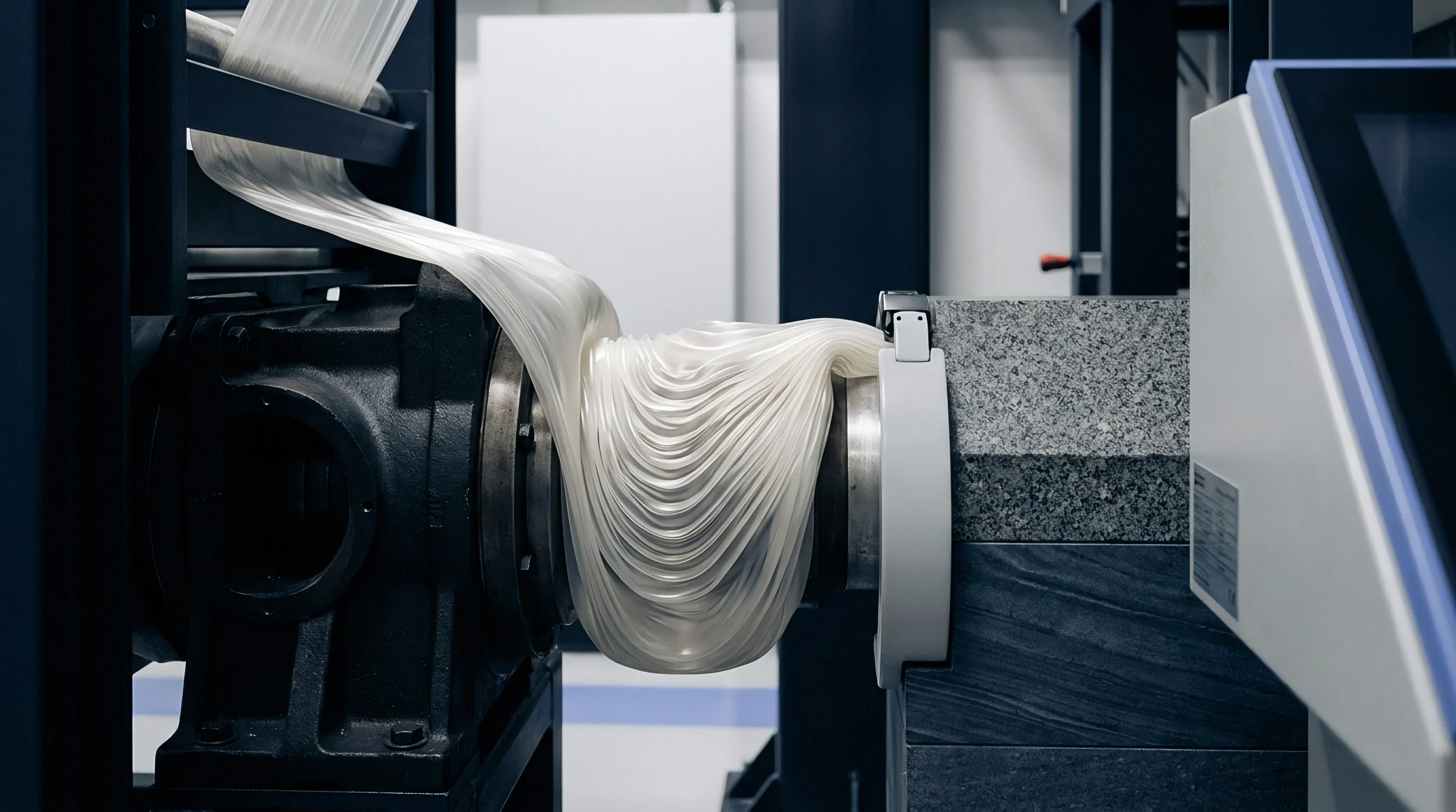
Simultaneous solution of mechanical and thermal domains remains necessary to capture interfacial detachment mechanics accurately. Thermomechanical interactions in injection molding operate as a continuous feedback loop. Thermal energy extraction drives volumetric shrinkage, generating internal stress fields that alter polymer mechanical strain.
Accumulated mechanical strain shifts the physical location of part boundary surfaces relative to tool steel, altering interfacial contact pressure and opening local air gaps. These gaps immediately reduce thermal contact conductance, altering heat flux vectors and shifting core cooling rates.
Thermomechanical Solvers and Gap Formation Dynamics
Implicit computational engines evaluate material displacement fields and thermal transport equations concurrently or through tightly coupled staggered iterations. Sequential uncoupled multiphysics approaches execute thermal solver steps first, exporting calculated nodal temperature histories into a secondary mechanical stress analysis. Uncoupled workflows fail to account for local gap creation during early cooling.
Uncalibrated models underpredict final warpage.
Tightly coupled solver schemes update the boundary conductance mesh matrix at every computational time step. When mechanical stress calculations indicate that local contact pressure between polymer boundary elements and cavity steel elements drops to zero, the solver reduces the interfacial heat transfer coefficient to its open-gap value. If thermal shrinkage causes mechanical detachment, the local gap clearance distance is computed directly.
Solvers modify conductance values based on radiative and conductive heat transport through the calculated air gap width, maintaining physics accuracy as part wall geometry warps inside the mold.
Thermomechanical strain detachment drops interfacial heat flux long before cavity pressure reaches atmospheric level.
Mesh density at cavity surface boundaries controls coupling accuracy. Coarse boundary element meshes blend interfacial pressure values over large surface areas, smoothing out localized pressure drop events. Fine boundary layer meshing, featuring at least five elements across the skin thickness domain, resolves steep temperature gradients and precise mechanical separation points.
Radial mesh refinement near complex geometry features, such as deep ribs and core pins, captures differential cooling vectors that drive localized part warpage.
| Coupling Architecture | Computational Speed Factor | Interface Boundary Updating | Warpage Prediction Accuracy | Convergence Stability |
|---|---|---|---|---|
| Decoupled Sequential | 1.0x (Baseline Fast) | Static Step Changes | Low (± 35% error) | Very High |
| Staggered Explicit-Implicit | 3.5x – 5.0x slower | Updated per Time Step | High (± 8% error) | Moderate (Mesh Sensitive) |
| Monolithic Fully Implicit | 12.0x – 20.0x slower | Continuous Field Mapping | Very High (± 3% error) | Low (Requires Dampened Steps) |
Stress Relaxation Interactions with Interfacial Heat Transfer
Viscoelastic polymer behavior modulates the mechanical force exerted against tool steel during the cooling phase. Amorphous and semi-crystalline resins exhibit time-dependent stress relaxation during packing and cooling. Peak hydraulic holding pressure generates high initial wall contact forces, but molecular stress relaxation reduces real boundary contact force even while internal cavity pressure remains elevated.
Thermomechanical solvers incorporating viscoelastic constitutive models, such as Williams-Landel-Ferry shift functions paired with Maxwell viscoelastic modes, calculate this contact force decay accurately.
Viscoelastic stress relaxation reduces effective thermal contact conductance prior to complete pressure release. As solidifying skin layers relax under continuous cooling, mechanical pressure transfer to cavity walls declines, lowering contact conductance before gate freeze occurs. Incorporating viscoelastic stress relaxation into solver parameter calibration prevents overestimating thermal transfer during late packing, refining predicted volumetric sink depth on aesthetic show surfaces.
Which computational boundary criteria best determine the exact threshold where mechanical mold deflection overcomes polymer holding pressure to open localized corner gaps?
Economics
Commercial viability in precision injection moulding hinges on reducing tool commissioning iterations and eliminating post-launch quality failures. Tooling capital deployed for multi-cavity production molds requires predictable return on investment, anchored by cycle time guarantees and dimensional compliance under drawing standards such as DIN 16742. Relying on uncalibrated multiphysics simulations introduces significant commercial risk, forcing toolmakers to re-machine hardened steel molds when production parts fail quality audits.
Tooling Sign off and Tolerancing Impact under Dynamic Cooling
Part drawings specified under strict geometric standards mandate tight tolerance bands on critical features. Achieving tolerance grades between TG3 and TG5 under DIN 16742 demands precise control over part shrinkage vectors. Uncalibrated solvers miscalculate pressure-dependent thermal conductance, leading to incorrect shrinkage allowances machined into tool cavities.
Steel modifications carry steep commercial costs.
When an uncalibrated solver underestimates thermal contact conductance during packing, predicted part shrinkage comes out lower than real production behavior. Toolmakers cut steel cavities too small based on flawed simulation output. Correcting this error requires EDM electrode machining, tool welding, or expensive rebuilds of core and cavity inserts.
Steel recutting cycles typically cost between eight thousand and twenty-five thousand dollars per tool modification pass, adding weeks to tool delivery timelines. Tool shop delays destroy production schedules.
Amortizing Calibration Expenses against Mold Modification Costs
Upfront financial investment in characterization protocols yields immediate capital protection across high-volume production programs. Conducting sensor-instrumented tool trials and running inverse solver calibration routines requires a baseline allocation of technical resources. Empirical calibration trials on a single-cavity test tool cost approximately twelve thousand to eighteen thousand dollars, covering sensor installation, charge amplifier hardware, press time, and engineering simulation hours.
Validated physics protect tooling capital.
Amortizing this single calibration fee across multiple tooling programs using identical resin grades reduces per-tool simulation validation expense to nominal levels. The financial return becomes clear when set against the costs of uncalibrated tool commissioning errors. Eliminating two tool modification loops on a high-cavity automotive or medical tool program recovers the calibration expenditure entirely, while protecting launch schedules and preventing contractual delivery default penalties.
Procurement agreements for complex multi-cavity injection tooling must include a mandatory clause requiring solver thermal boundary conditions to be calibrated against flush-mounted transducer data before finalizing cavity steel dimensions.