Interfacial Heat Transfer Coefficient Calibration Using In-Cavity Pressure and Temperature Sensors
Calibrating dynamic interfacial heat transfer coefficients with flush cavity sensors eliminates cooling simulation error and prevents unbudgeted cycle time extensions.

Flux
Injection moulding simulation software historically treats heat extraction as a uniform, static boundary condition across mold surfaces. Polymer thermal contact resistance varies continuously throughout the injection, packing, and cooling phases. Precise thermal modeling depends on calculating the interfacial heat transfer coefficient as a dynamic function of localized pressure, temperature, and spatial clearance between the cooling polymer skin and cavity steel.
Mechanics of Polymer Steel Contact Heat Flux
Rapid cavity filling brings high-temperature molten resin into intimate physical proximity with chilled cavity tooling. During initial melt injection, extreme wall shear rates and high delivery pressures force polymer chains into microscopic surface rough asperities along the tool wall. Melt contact governs heat flow.
This intimate mechanical coupling minimizes interfacial air pockets, driving boundary conductance values to peak levels during the high-pressure filling and packing stages.
Heat extraction across the boundary obeys basic conduction principles modified by thermal contact resistance:
q” = h_i (T_skin – T_wall)
Where q” represents local heat flux, T_skin represents polymer surface temperature, T_wall represents cavity steel surface temperature, and h_i represents the dynamic interfacial heat transfer coefficient. As cavity pressure escalates during the holding phase, microscopic gap compression increases real contact area, driving h_i toward its theoretical upper limit.
Phase Dependent Resistance from Fill to Detachment
Pressure drops rapidly once gate freeze limits continuous packing flow from the machine nozzle. Volumetric shrinkage causes the cooling polymer matrix to contract away from the cavity walls. This physical contraction creates a microscopic air gap between the solidifying polymer skin and the mold steel.
Air acts as an insulator. The thermal conductivity of trapped cavity gas sits near 0.026 Watts per meter Kelvin, roughly three orders of magnitude lower than tool steel. The onset of physical gap detachment causes interfacial conductance to plummet.
Thermal conductance falls. Managing this transition requires empirical calibration rather than fixed coefficient assumptions in computer-aided engineering software.
High clamping pressure suppresses interfacial gas gaps, elevating thermal contact conductance during the holding phase.
| Process Phase | Pressure Range (bar) | Interfacial State | Representative IHTC (W/m²K) |
|---|---|---|---|
| Filling Phase | 200 – 800 | Pressurized viscous contact with surface asperities | 1500 – 2200 |
| Packing Phase | 400 – 1200 | Maxed mechanical coupling and compressed interface | 2000 – 3500 |
| Cooling Phase (Pre-Detachment) | 50 – 300 | Solidified skin maintaining intimate contact under residual pressure | 800 – 1400 |
| Post-Detachment Phase | 0 – 10 | Microscopic air gap formation due to volumetric shrinkage | 100 – 350 |
Higher packing pressures maintain physical wall contact longer into the cycle, delaying thermal insulation caused by part detachment.
Probe
Piezoelectric pressure transducers and rapid-response surface thermocouples mounted in cavity steel capture real-time boundary state changes. Accurate calibration of heat transfer coefficients relies directly on synchronizing high-frequency temperature transients with instantaneous cavity pressure traces.
In Cavity Sensor Architecture and Transient Response
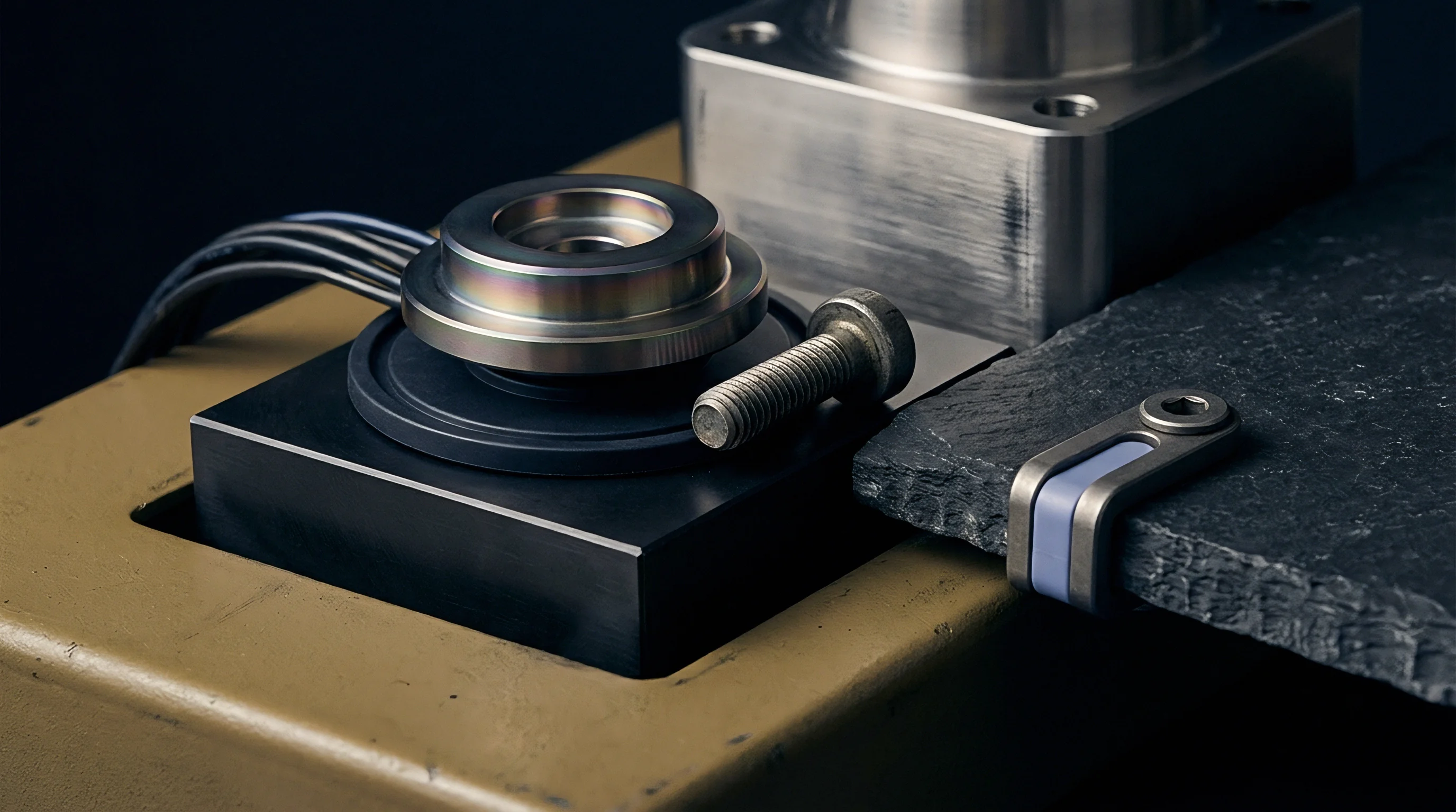
Dual-function instrumentation combining quartz crystal elements and coaxial thermocouples provides simultaneous local physical traces. Installing sensors flush with the cavity wall prevents flow front distortion while capturing localized skin temperature spikes occurring within milliseconds of melt arrival. Sensor placement targets high-sensitivity zones including the gate location, mid-flow path, and end-of-fill region.
Fast sampling rates are mandatory for inverse thermal calculations. Data acquisition hardware recording at minimum frequencies of one kilohertz captures sharp initial thermal gradients. Thermocouples constructed with thin-film junctions positioned within micrometers of the cavity surface deliver response times under two milliseconds, avoiding time-lag smoothing that corrupts peak heat flux derivations.
At cavity pressure exceeding 600 bar, interfacial heat transfer coefficient reaches peak values near 2500 Watts per square meter Kelvin.
Signal Distortion Sources in Tool Steel Installation
Machining tolerances for transducer pockets directly dictate data accuracy. Sensor alignment determines data accuracy. A transducer recessed by as little as twenty micrometers creates a stagnant polymer pocket that acts as a thermal insulator, artificially lowering calculated heat flux values.
Conversely, a protruding sensor acts as a flow obstruction, introducing localized shear heating spikes.
Improper torque damages fragile ceramic seals. Sensor installation guidelines require calibrated torque wrenches to prevent mounting pocket distortion and piezoelectric element prestress shifts.
- Sensor Tip Recess Creates a stagnant polymer melt pocket that distorts local pressure transmission and introduces thermal time delays.
- Thermocouple Sheath Insulation Dampens fast thermal transients during high-speed cavity filling, yielding artificially suppressed heat flux estimates.
- Piezoelectric Preload Drift Alters voltage output under continuous high-temperature cycling, corrupting pressure-dependent heat transfer decay mappings.
- Cable Impedance Shifts Introduces high-frequency noise during rapid cavity pressure decay, distorting mathematical inversion routines.
Uncorrected sensor offset errors propagate through thermal boundary equations, leading to incorrect cooling time projections that force tool shop modification rework.
Scheme
Mathematical reconstruction converts raw sensor voltage streams into boundary heat loss rates. Determining interfacial heat transfer coefficients requires solving the Inverse Heat Conduction Problem, calculating unknown boundary conditions from transient interior or surface temperature measurements.
Mathematical Formulations for Inverse Heat Conduction
Solving the governing heat equations backwards requires numerical stabilization due to inherent mathematical instability. Experimental measurement noise in thermocouple signals amplifies dramatically during inverse differentiation. Beck’s sequential function specification method stabilizes the solution by utilizing future time steps to predict current boundary heat flux.
Numerical solvers demand precise inputs. The mathematical relationship governing pressure-dependent and gap-dependent heat transfer combines piecewise functions:
h_i(P) = h_max (P / P_ref)^n
When cavity pressure drops to zero, the formulation switches to an air-gap conductance model where clearance distance d(t) is derived from volumetric shrinkage models:
h_i(d) = k_air / d(t) + sigma (T_skin^2 + T_wall^2) (T_skin + T_wall) / (1/epsilon_p + 1/epsilon_m – 1)
Conduction slows after gap formation. Radiation heat transfer terms contribute minimally at standard polymer processing temperatures but gain importance in high-temperature engineering thermoplastics such as polyetheretherketone.
Are Transient Surface Temperature Spikes Representative of Bulk Polymer Cooling?
Surface thermocouple records capture boundary contact skin effects rather than core cross-section thermal distributions. Skin temperature fluctuations reflect instantaneous local heat flux, but bulk polymer core cooling rates depend heavily on thermal diffusivity across the entire wall thickness. Calibration algorithms must reconcile localized surface sensor dynamics with one-dimensional or three-dimensional heat conduction equations across the polymer thickness.
- Data acquisition hardware records synchronized time-series vectors for cavity pressure P(t) and mold surface temperature T(t) during a stable molding trial.
- A finite element model of the mold steel domain applies recorded surface temperature traces as transient Dirichlet boundary conditions.
- The inverse algorithm calculates transient heat flux q”(t) by minimizing error residuals between measured and predicted steel temperatures.
- Parameter fitting software regresses non-linear empirical coefficients mapping calculated heat flux against coincident cavity pressure values.
- An air-gap clearance model incorporates calculated thermal shrinkage to establish post-detachment heat transfer coefficients.
Calibrated decay coefficients eliminate numerical divergence in cooling simulations when air gap formation initiates during post-fill shrinkage.
| Resin Family | Morphology | Peak Pressure (bar) | h_max (W/m²K) | Pressure Exponent n | Detachment Gap IHTC (W/m²K) |
|---|---|---|---|---|---|
| Polypropylene (PP) | Semi-crystalline | 600 | 2800 | 0.42 | 120 |
| Polycarbonate (PC) | Amorphous | 800 | 2100 | 0.31 | 180 |
| Polyamide 66 (PA66) | Semi-crystalline | 750 | 3100 | 0.48 | 100 |
| Acrylonitrile Butadiene Styrene (ABS) | Amorphous | 500 | 1950 | 0.28 | 160 |
Whether non-linear polymer viscosity changes during local flow stagnation alter boundary thermal impedance remains an open research question across multi-cavity tooling designs.
Trial
Validating simulation boundary parameters demands structured DOE runs on a production press. Empirical calibration requires isolating holding pressure, melt temperature, and mold wall temperature variables across controlled tool trials.
Scientific Tool Trial Execution for Empirical Data Generation
Press settings vary systematically across melt temperature, mold wall temperature, and holding pressure levels. Press settings dictate thermal boundary behavior. Systematically stepped holding pressure levels alter wall contact duration, yielding distinct pressure-temperature curves for inverse solver processing.
Data collection demands high rates. Transducers stream pressure and temperature values into external signal conditioning hardware while machine controllers record screw position and hydraulic pressure. Standardizing cycle step timing eliminates thermal equilibrium shifts between test shots.
Cross Validation against Physical Part Shrinkage and Warpage
Computed heat transfer profiles feed directly into warp prediction codes to evaluate geometric accuracy against molded samples. Imparting realistic boundary cooling rates improves volumetric shrinkage predictions. Core temperature pyrometers verify simulation accuracy.
Physical part dimensions measured via coordinate measuring machines check simulation warp output against actual molded parts. Standard DIN 16742 tolerance classes serve as baseline target metrics for empirical validation runs.
- Boundary Flux Verification Checks that measured pressure decay mirrors cavity temperature inflection points across all gating zones.
- Gap Conductance Threshold Mapping Verifies that predicted part detachment aligns with physical core temperature plateaus observed during ejection.
- Resin Viscosity Correlation Isolates thermal contact resistance from melt viscosity variations during variable holding pressure trials.
- Cooling Channel Reynolds Number Control Audits water flow rate to confirm cavity wall temperature remains invariant during high-heat transients.
Toolmakers often attribute unexpected sink marks or dimensional drift to resin batch variation rather than uncalibrated boundary thermal assumptions.
Charge
Capital investments in multi-cavity tooling depend directly on predicted cooling cycle seconds. Simulation software using default heat transfer coefficients frequently underestimates required cooling times, distorting tooling ROI calculations and machine scheduling capacity plans.
Tooling Budget Impact of CAE Default Assumptions
Software default heat transfer values frequently underestimate required cooling times by fifteen to twenty percent. Simulation errors raise costs. Assuming a constant interfacial heat transfer coefficient of 1200 Watts per square meter Kelvin oversimplifies physical reality, masking long cooling delays caused by early part detachment gap thermal insulation.
Cooling dominates total cycle time. In automotive or medical packaging tooling, two seconds of unpredicted cooling delay adds massive operational costs over production lifetimes.
Consider a 32-cavity polypropylene medical closure tool running on an automated press. Simulation using uncalibrated default heat transfer coefficients predicts a 7.5-second cooling cycle, yielding an 11.0-second total cycle time. Production trials reveal that early part detachment causes heat retention in thick thread sections, forcing setters to extend cooling time to 9.5 seconds to hold DIN 16742 tolerance Grade TG6.
Cycle savings compound across high production volumes. An unpredicted 2.0-second cycle extension on an annual volume of 50 million parts increases press operating time by over 270 hours, consuming an unbudgeted 35,000 USD in press machine-hour charges.
| Parameter / Metric | Default CAE Assumption | Calibrated IHTC Simulation | Variance / Impact |
|---|---|---|---|
| Assumed IHTC Model | Constant 1200 W/m²K | Dynamic P(t) and Gap Dependent | Physically realistic heat extraction |
| Predicted Cooling Time | 7.5 seconds | 9.4 seconds | +1.9 seconds predicted prior to steel cut |
| Cooling Circuit Design | Standard drilled lines | Conformal cooling inserts | Modifies tooling capital expenditure |
| First Article Sample Approval | Failed warp check at T1 | Passed dimensional audit at T1 | Eliminates 2 tool tuning iterations |
| Tooling Rework Expense | 18,500 USD | 0 USD | Direct capital expenditure savings |

Contractual Verification Provisions for Tool Acceptance
Purchase specifications require documented cavity pressure and temperature calibrations before sign-off. Tool procurement contracts increasingly incorporate mandatory thermal validation dossiers to guarantee that quoted cycle times reflect press-side realities.
- Calibrated Parameter Matrix Maps pressure and gap distance to heat flux transfer values for specific polymer grades.
- Sensor Calibration Certificates Provides traceability records for all piezoelectric pressure transducers and thin-film thermocouples used in calibration trials.
- Raw Signal CSV Records Supplies time-series data for pressure and temperature acquired at minimum one-kilohertz sampling rate during tool trials.
- Simulation Deviation Ledger Quantifies variance between predicted core cooling rates and physical pyrometer measurements prior to final tool sign-off.
ISO 20753 thermal test clauses mandate documented verification of boundary cooling parameters before tool release approval.
Standard tool procurement contracts invoking DIN 16742 dimensional compliance shift heat transfer calibration costs to the toolmaker if first-article samples fail thermal cooling audits.