Deriving Ogden Constitutive Parameters from Biaxial Stretch Testing Data
Deriving Ogden constitutive parameters pairs non-linear biaxial stretch data with Drucker stability constraints to ensure reliable finite element simulations.


Rig
Biaxial tension frames use four motor arms on two orthogonal axes to pull sheet specimens into planar stress states. Characterizing hyperelastic polymers requires tracking load and displacement on both axes simultaneously. Standard uniaxial test frames create a simple one-dimensional strain field that misses the multi-axial strain hardening and stress relaxation occurring in thermoforming, stretch-blow molding, or diaphragm inflation.
Controlling the displacement rate ratio between axes allows biaxial frames to isolate non-linear material response across equal biaxial, unequal biaxial, and planar stretch modes.
Specimen geometry determines how uniform the central strain field remains during testing. Cruciform samples cut from extruded or calendered sheet feature a central gage section bounded by four arms. Machining slits along these arms cuts down shear transfer from rigid grips into the measurement zone.
The grips must clamp tight enough to prevent slippage without creating stress concentrations that tear the specimen at the boundary. Pneumatic or hydraulic grips with serrated or elastomeric faces maintain consistent pressure along each arm, while scissor linkages keep the specimen center aligned with the optical center during asymmetrical pulls.

Biaxial Testing Hardware and Specimen Geometry
Cutting cruciform samples from extruded sheet provides a central gage area surrounded by four loading arms. Longitudinal slots machined in each arm relax lateral constraints, allowing the central zone to expand naturally along both axes without artificial stiffening from the boundaries. Load cells on each actuator spindle record forces individually, making off-center drift or grip slip immediately visible.
Opposing grips are aligned within 0.05 millimeters to keep unwanted shear couples from altering the data.
The dimensions of the central square set the upper limit on stretch before the arms fail. Machining or molding a slight relief into the center concentrates deformation within the optical measurement area, protecting the arm fillets from early rupture. For elastomeric sheet between 1.0 and 3.0 millimeters thick, a 20 millimeter by 20 millimeter reduced gage section maintains a uniform biaxial stress state beyond stretch ratios of 4.5.
Grip speed sets the engineering strain rate, usually kept between 0.01 and 10 reciprocal seconds to map rate-dependent behavior.
Biaxial strain fields measured via optical digital image correlation maintain true strain accuracy within 0.002 units across sample velocities between 1 and 500 millimeters per second.
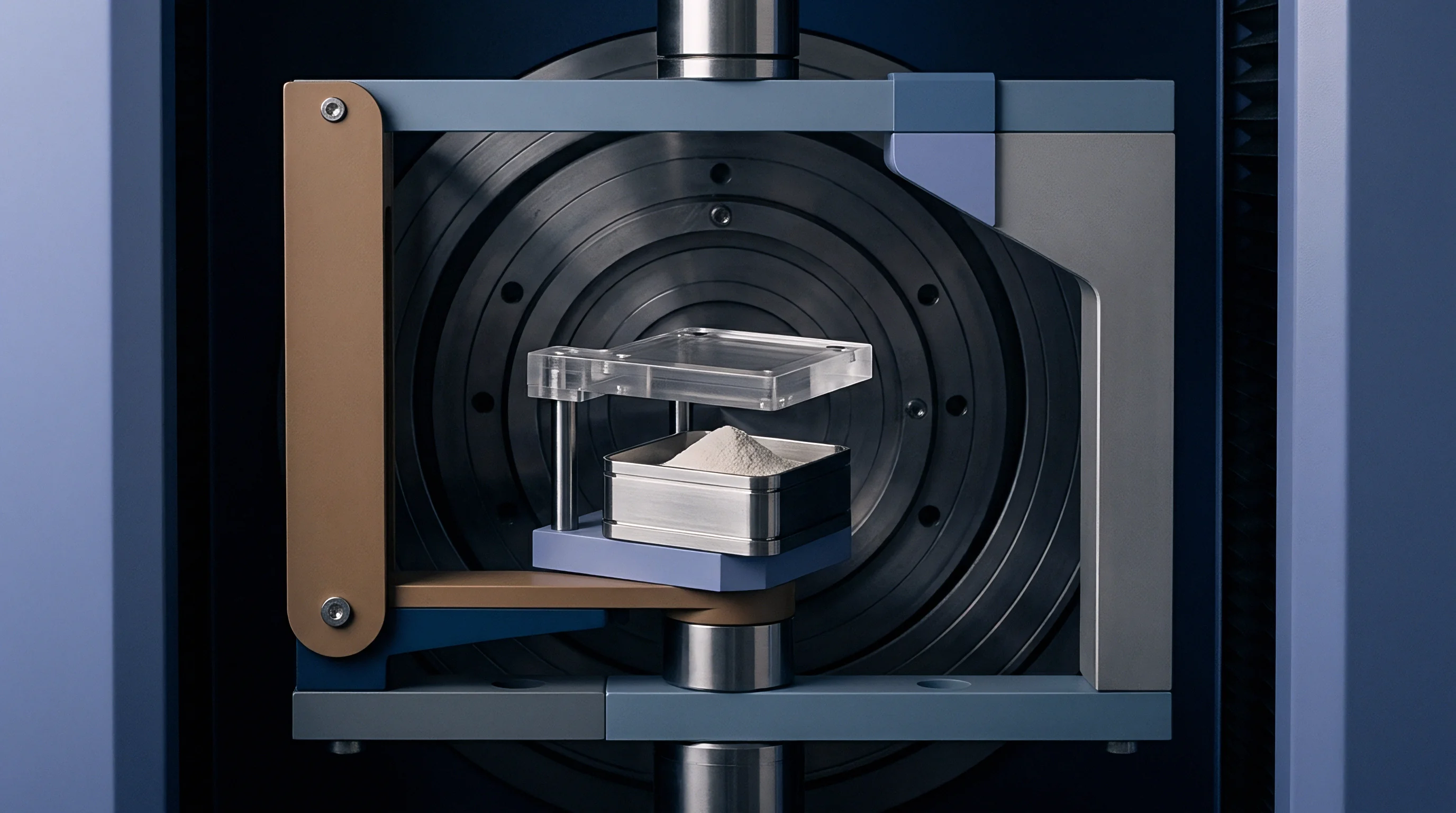
Optical Strain Tracking Mechanics
Non-contact displacement tracking relies on high-resolution digital cameras focused on a high-contrast random speckle pattern on the gage surface. Digital Image Correlation software calculates the spatial deformation gradient tensor by tracking sub-pixel shifts across sequential frames. Encoder readings from actuator cross-heads overestimate strain because of frame compliance and grip-zone stretching.
Computing strain optically from the central gage area removes hardware compliance from the material equations.
Stereo camera pairs capture out-of-plane deflections at high stretch levels. As the sheet thins rapidly under stretch, calculating true Cauchy stress from load cell data requires updating the cross-sectional area in real time. Dual-camera setups resolve 3D surface coordinates down to sub-micron resolution.
Standard calibration grids establish focal lengths, distortion parameters, and camera angles before testing begins.
- Cruciform arm slotting keeps edge constraint from restricting lateral expansion across the central optical gage area.
- Pneumatic grip pressure tracking prevents specimen slippage artifacts from skewing load records at high stretch ratios.
- Scissor-frame centering alignment prevents the specimen center from shifting during unequal biaxial extension.
- Random speckle pattern density preserves spatial contrast under extreme stretching without paint cracking or flaking.

Environmental Control for Thermoforming States
Heated environmental chambers maintain uniform temperatures across the sample during elevated-temperature tests. Thermoforming and stretch-blow molding operate well above room temperature ~ typically between 120 and 160 degrees Celsius for amorphous polymers like poly(methyl methacrylate) or poly(ethylene terephthalate). Forced-convection chambers with optical glass windows permit full DIC tracking while keeping gage temperature swings within 0.5 degrees Celsius.
The specimen must reach thermal equilibrium before testing. A soak time of 180 to 300 seconds ensures the sheet heats uniformly through its thickness. Infrared sensors verify surface temperatures across the arms and gage area, while radiant panels above and below the specimen react to offset heat loss near optical viewing ports.
When labs run into uneven central strain fields during high-speed tests, suppliers often trace the issue back to sheet anisotropy from extrusion rather than jaw synchronization error.


Strain
Analyzing hyperelastic deformation relies on principal stretch ratios measured along orthogonal axes. The deformation gradient tensor translates spatial tracking points into strain values. For uniform planar deformation, this tensor reduces to a diagonal matrix aligned with the principal stretch directions.
Assuming incompressibility simplifies kinematics further by linking out-of-plane stretch directly to the product of the two in-plane stretches.
Ogden constitutive models define hyperelastic behavior using principal stretch values directly rather than strain invariants. Raymond Ogden structured this strain energy potential as a linear combination of principal stretch powers, capturing non-linear behavior in soft elastomers, biological tissues, and uncrosslinked polymer melts. The resulting strain energy density function sums a fixed number of modulus-exponent parameter pairs.
Principal Stretch Relationships and Incompressibility
Kinematically, stretch ratio is current length divided by original length along a principal axis. Denoting the optically measured in-plane stretches as lambda one and lambda two, the deformation gradient tensor maps reference positions to deformed coordinates. Its scalar determinant measures local volume change.
At moderate hydrostatic pressures, polymers experience virtually no volume change, making the incompressible assumption realistic. Setting the determinant to unity makes the out-of-plane stretch equal to the inverse product of the two in-plane stretches. This constraint drops volumetric strain terms from the formulations, allowing sheet thinning calculations directly from surface DIC data.
ISO 16938 compliance demands independent measurement of orthogonal axes to prevent shear strain artifacts from altering derived strain energy densities.

Ogden Strain Energy Density Formulation
Raymond Ogden’s potential expresses energy density purely through principal stretches, summing non-integer power terms composed of a shear modulus coefficient and a strain-hardening exponent. For an incompressible material, the potential takes this form:
W = sum from i=1 to N of (mu_i / alpha_i) (lambda_1^(alpha_i) + lambda_2^(alpha_i) + lambda_3^(alpha_i) – 3)
Here, the parameters mu_i are shear moduli in megapascals, and alpha_i are dimensionless strain-hardening exponents. The model order N is usually set between 1 and 3 for finite element implementation. At infinitesimal strains, the initial shear modulus equals half the sum of the products of mu_i and alpha_i across all terms.
Grounding Ogden parameters in physical test data demands mapping raw measurements through specific kinematic relationships:
- Position optical digital image correlation targets across the central gage area of the cruciform specimen.
- Apply synchronous motor drive profiles to pull orthogonal axes at fixed velocity ratios representing equal biaxial or planar stretch.
- Record nominal force signals from all four inline load cells continuously throughout the displacement sequence.
- Compute in-plane principal stretches lambda one and lambda two directly from spatial coordinates of tracked speckle clusters.
- Calculate out-of-plane stretch lambda three using the incompressibility constraint lambda three equals the inverse product of lambda one and lambda two.
- Determine true Cauchy stresses by dividing measured forces by the instantaneous deformed cross-sectional areas along each axis.
- Convert Cauchy stress components to nominal engineering stress values for objective function residual evaluation.

Stress Field Derivations across Biaxial Modes
Differentiating the strain energy function with respect to principal stretch yields stress expressions along each axis. Because the material is incompressible, the Cauchy stress includes an unknown hydrostatic pressure term. Setting the out-of-plane stress to zero ~ matching thin-sheet plane stress conditions ~ eliminates this hydrostatic pressure scalar.
True principal stress along direction one is the stretch derivative multiplied by the stretch component minus hydrostatic pressure. Substituting the pressure term derived from the zero out-of-plane stress boundary condition gives the Cauchy stress along direction one:
sigma_1 = sum from i=1 to N of mu_i (lambda_1^(alpha_i) – (lambda_1 lambda_2)^(-alpha_i))
Stress along direction two follows by symmetry. Nominal engineering stresses, defined as current force divided by initial area, relate back to true Cauchy stresses through multiplication by the inverse of the principal stretch ratio.
| Deformation Mode | In-Plane Stretch 1 | In-Plane Stretch 2 | Out-of-Plane Stretch 3 | Principal Cauchy Stress Difference |
|---|---|---|---|---|
| Uniaxial Extension | lambda | lambda^(-0.5) | lambda^(-0.5) | sigma_1 = sum mu_i (lambda^(alpha_i) – lambda^(-0.5 alpha_i)) |
| Equal Biaxial Extension | lambda | lambda | lambda^(-2) | sigma_1 = sum mu_i (lambda^(alpha_i) – lambda^(-2 alpha_i)) |
| Planar Extension (Pure Shear) | lambda | 1.0 | lambda^(-1) | sigma_1 = sum mu_i (lambda^(alpha_i) – lambda^(-alpha_i)) |
| Unequal Biaxial Extension | lambda_1 | lambda_2 | (lambda_1 lambda_2)^(-1) | sigma_1 = sum mu_i (lambda_1^(alpha_i) – (lambda_1 lambda_2)^(-alpha_i)) |
Single-mode tensile data cannot adequately constrain hyperelastic model behavior under multi-axial processing conditions.

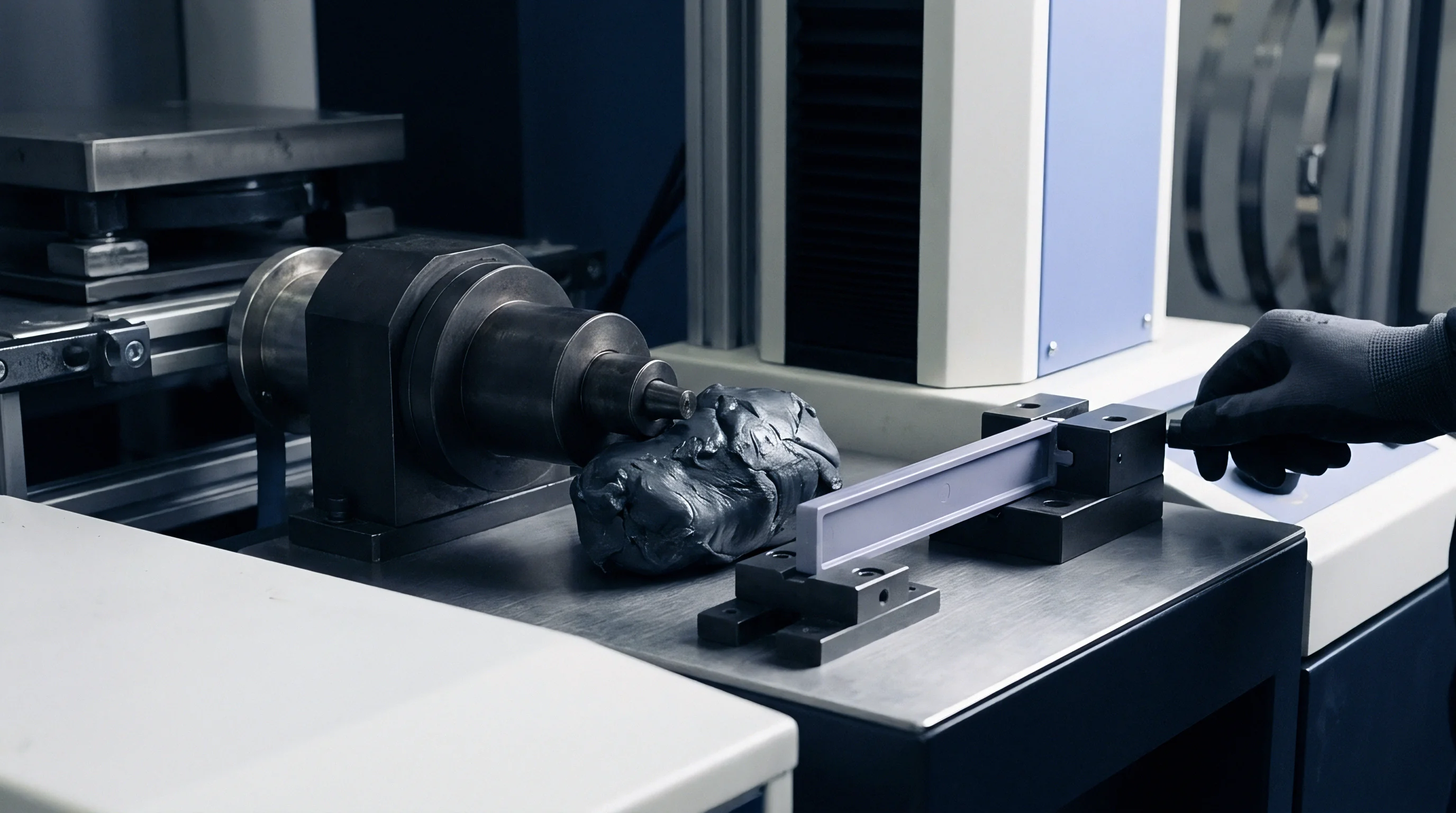
Regression
Fitting constitutive parameters to stress-stretch data relies on non-linear least squares algorithms to minimize residual errors. To obtain robust parameters, experimental curves from uniaxial, equal biaxial, and planar stretch modes must feed into the objective function simultaneously. Regressions based on single-mode data might fit one curve well, but they often diverge under multi-axial loading.
The objective function must account for differences in stress magnitude across modes. At equal stretch ratios, biaxial stresses are often three times higher than uniaxial stresses. Unweighted least-squares fitting naturally favors high-stress biaxial points while ignoring low-strain uniaxial or planar data.
Weighting by relative error normalizes these differences, maintaining fitting quality across the full strain range.

Non-Linear Least Squares Optimization Routines
Fitting hyperelastic curves requires optimization algorithms capable of handling non-convex parameter landscapes. Levenberg-Marquardt is standard, combining gradient descent stability with Gauss-Newton convergence. Global search methods like genetic algorithms or particle swarm optimization often run first to locate good starting neighborhoods, preventing local gradient solvers from stalling in local minima.
Sensitivity analyses show strong coupling between Ogden term pairs. Small changes in alpha exponents produce non-linear shifts in mu coefficients, causing ill-conditioned Hessian matrices during gradient steps. Setting explicit parameter bounds keeps shear moduli positive and restricts alpha exponents to realistic limits, usually between -15 and +15.
Parameters fitted exclusively to uniaxial extension fail when predicting hyperelastic response under multi-axial inflation loading.
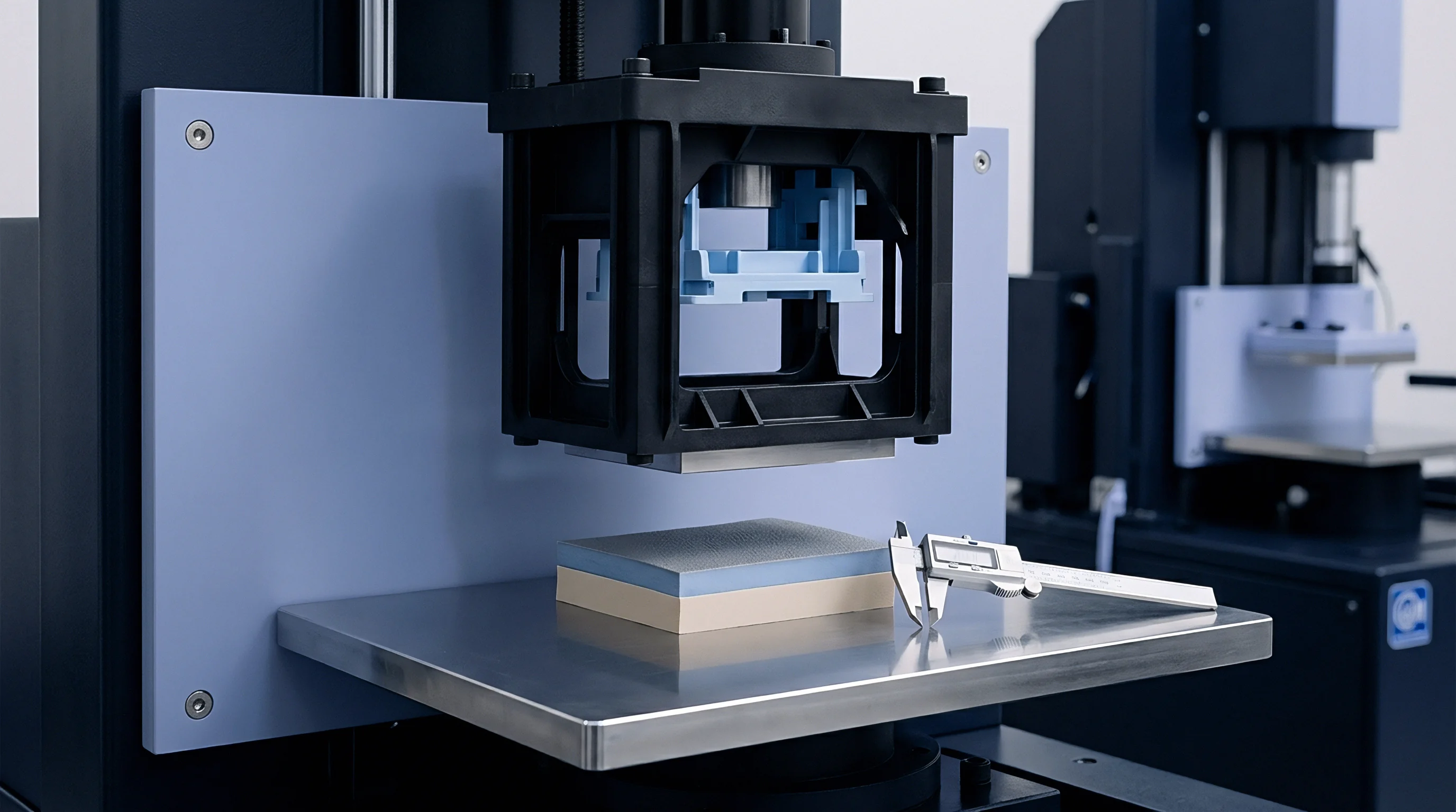
Drucker Stability Constraints and Matrix Conditioning
To converge in implicit finite element solvers, hyperelastic models must maintain a positive definite tangent stiffness tensor under multi-axial loads. Drucker stability requires that any incremental stress step performs positive work along an incremental strain path. Mathematically, the second-derivative matrix of the strain energy density potential must retain positive eigenvalues across all expected stretch states.
For an incompressible Ogden material, initial stability requires the sum of mu_i times alpha_i to be strictly positive, and individual term pairs generally should meet the same condition. Regression routines evaluate stability at every iteration, penalizing unstable parameter candidates to keep the optimizer within physically sound regions.
Decision criteria for configuring parameter fitting schemes include:
- Relative error normalization weighting prevents high-magnitude biaxial stress data points from dominating low-strain uniaxial residual evaluations.
- Drucker stability penalty functions reject parameter candidates that exhibit negative tangent stiffness values within the targeted stretch domain.
- Lower-bound modulus inequality constraints enforce strictly positive initial shear stiffness contributions across every Ogden term pair.
- Multi-mode residual pooling combines uniaxial, equal biaxial, and planar stretch datasets into a single simultaneous objective function.

Order Selection and Numerical Convergence
Selecting the number of terms in the Ogden series involves balancing curve fit accuracy against solver stability. A first-order model (N=1) offers basic hyperelastic response but misses the S-shaped inflection typical of filled elastomers or strain-crystallizing polymers. A second-order model (N=2) captures non-linear softening and moderate strain hardening.
Third-order models (N=3) provide excellent fidelity over wide strain ranges, tracking steep upturns prior to rupture.
Expanding to four or more term pairs introduces mathematical instability. Parameter ill-conditioning increases rapidly, causing unphysical stress oscillations between experimental data points. In finite element runs, these artificial stiffness spikes lead to element inversion and convergence failures.
Second- or third-order models generally offer the best compromise between fit accuracy and numerical reliability.
| Model Order (N) | Number of Parameters | Uniaxial Residual Error (%) | Biaxial Residual Error (%) | Drucker Stability Compliance |
|---|---|---|---|---|
| N = 1 (Mooney-Rivlin Equiv) | 2 (mu_1, alpha_1) | 8.4 | 12.1 | Unconditionally Stable |
| N = 2 | 4 (mu_1-2, alpha_1-2) | 2.1 | 3.2 | Stable across stretch < 5.0 |
| N = 3 | 6 (mu_1-3, alpha_1-3) | 0.6 | 1.1 | Requires explicit constraints |
| N = 4 | 8 (mu_1-4, alpha_1-4) | 0.3 | 0.8 | Prone to non-physical oscillations |
Applying single-mode uniaxial fit parameters to an equal-biaxial stretch-blow molding model introduces a 14 percent deviation in predicted sheet wall thickness.
Improper residual weighting during optimization produces parameter sets that trigger convergence aborts in non-linear FEA solvers.

Divergence
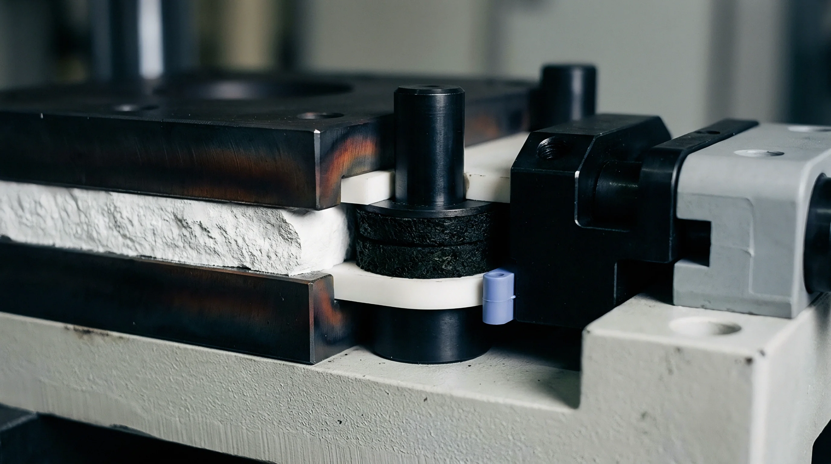
Experimental stretch data often departs from ideal predictions because of hysteresis and strain history. Under cyclic loading, polymer sheets exhibit energy dissipation from the Mullins effect. Unfilled elastomers and TPOs show noticeable stress softening during early cycles, requiring pre-conditioning to obtain repeatable curves.
Fitting models to virgin first-stretch data overestimates material stiffness for subsequent forming steps.
Extrusion anisotropy represents another common source of divergence. Polymer chain alignment along the machine direction makes the sheet stiffer along that axis than in the transverse direction. Isotropic Ogden formulations assume identical properties in all directions.
When fitted to anisotropic data, the regression averages out directional differences, underpredicting machine-direction stiffness and overpredicting transverse stiffness.

Material Anisotropy and Mullins Softening Effects
Extruded or calendered sheets carry directional properties from processing. Comparing uniaxial curves at zero, forty-five, and ninety degrees to the extrusion axis reveals the degree of anisotropy. If orthogonal stresses differ by more than five percent at the same stretch ratio, standard isotropic models introduce systematic errors.
Highly anisotropic sheets require specialized formulations, such as Holzapfel-Gasser-Ogden models, rather than isotropic Ogden laws.
Pre-conditioning removes transient Mullins softening from the test dataset. Cycling cruciform specimens five times up to the peak expected stretch ratio stabilizes the polymer network. Fitting parameters to the sixth loading curve yields coefficients that accurately reflect material response during repeated forming or diaphragm operation.

Why Do Higher Order Ogden Models Predict Unphysical Stiffness?
High-order expansions with three or four term pairs fit noisy data closely, but unconstrained optimization can allow negative alpha exponents combined with large positive mu values to corrupt local gradient calculations. In stretch regions where test points are sparse, the model can produce artifacts like negative tangent moduli or artificial stiffness spikes.
When high-order parameters run in non-linear FEA solvers, elements entering unmapped strain regimes trigger immediate matrix ill-conditioning. Localized softening followed by abrupt artificial stiffening sends Newton-Raphson iterations into non-converging loops. Limiting Ogden regressions to N=2 or N=3 with strict Drucker constraints prevents solver divergence while maintaining fit quality across complex stretch paths.
Nonlinear regression algorithms require lower bound constraints on shear modulus terms to prevent negative strain energy density states in solver iterations.

Strain Rate Sensitivity in High-Speed Process Windows
Blow molding and vacuum forming deform sheet material at strain rates well above fifty reciprocal seconds. Quasi-static tests run at 0.01 reciprocal seconds isolate hyperelastic response but miss rate-dependent viscoelastic contributions. Using quasi-static parameters in high-speed simulations underestimates initial resistance, leading to incorrect inflation pressure and thickness predictions.
Accurate high-speed simulations require rate-dependent characterization and visco-hyperelastic models. Testing across three to four orders of magnitude in velocity maps rate sensitivity. Visco-hyperelastic formulations combine an instantaneous Ogden potential with a Prony series relaxation kernel, capturing strain-rate hardening, adiabatic heat softening, and stress relaxation during cooling.
How far can hyperelastic parameters derived from quasi-static biaxial tests be trusted when predicting high-speed thermoforming wall thinning across sharp tool corner radii?

Mesh
Simulating hyperelastic forming involves loading material parameters into solver material definition cards. Packages like Abaqus, ANSYS, and LS-DYNA use derivatives of the strain energy density function to build element stiffness matrices. Correctly converting units, parameter order, and volumetric terms ensures virtual press trials match physical test results.
Material incompressibility presents numerical challenges in non-linear FEA. Standard displacement-based solid elements lock up artificially when modeling near-incompressible response. Hybrid element formulations address this by assigning an independent hydrostatic pressure degree of freedom to each node, decoupling pressure from displacement derivatives and preventing locking in deep-draw regions.
Finite Element Solver Implementation Procedures
Transferring material coefficients into software like Abaqus or ANSYS requires strict unit consistency. Ogden shear moduli mu_i carry stress units and must align with the global model’s stress scale, while dimensionless alpha exponents remain unchanged. Entering MPa-based parameters into a millimetric system expecting pascals throws element stiffness off by six orders of magnitude.
Compressibility settings must be explicitly defined in the material card. While basic theory assumes absolute incompressibility, solvers need a finite bulk modulus to avoid singular matrices during setup. Setting a Poisson ratio between 0.4990 and 0.4995 introduces slight compressibility, balancing realistic volume preservation with numerical stability.
Element Formulation and Volumetric Incompressibility
Solid elements for hyperelastic analysis rely on mixed pressure-displacement formulations. First-order hybrid solids (like Abaqus C3D8RH) interpolate constant pressure across the element, preventing locking at high stretch ratios. Second-order hybrid elements yield smoother stress results along curved tool radii, though they are more sensitive to mesh distortion during deep drawing.
Membrane elements save computation time in thin-sheet forming where bending stiffness is negligible compared to tension. They compute in-plane stretch directly and update element thickness using the incompressibility constraint. For shell formulations, transverse shear options should be enabled to capture out-of-plane shear as the sheet wraps around tight radii.
- Unit system conversion verification ensures shear moduli match global finite element solver pressure and displacement dimension scales.
- Compressibility coefficient selection maintains Poisson ratios near 0.499 to prevent volumetric locking without causing matrix ill-conditioning.
- Hybrid element formulation assignment decouples hydrostatic pressure degrees of freedom from spatial node displacement vectors.
- Adaptive remeshing trigger configuration regenerates distorted mesh structures during extreme deep-draw sheet stretch steps.

Process Simulation and Thickness Prediction
Sheet inflation models map local thinning across tool cavities during vacuum forming. In these simulations, hyperelastic elements contact tool surfaces, transferring heat and altering local friction conditions. Well-fitted Ogden parameters reproduce bubble expansion accurately, predicting localized thinning, web formation limits, and corner thickness distributions.
Mismatches between simulated and actual part thickness usually point to poor material model choice. Parameters fitted only to uniaxial data underestimate resistance to multi-axial stretching, causing FEA models to overpredict thinning at dome centers. Using parameters fitted to multi-mode data resolves these errors, allowing tool designers to optimize preforms and plug profiles before machining steel.
| Tool Geometry Zone | Draw Ratio | Uniaxial Fit Error (%) | Equal Biaxial Fit Error (%) | Multi-Mode Ogden Fit Error (%) |
|---|---|---|---|---|
| Flat Base Center | 1.5 : 1 | 14.2 | 8.1 | 1.2 |
| Vertical Sidewall | 2.5 : 1 | 18.6 | 11.4 | 2.1 |
| Internal Corner Radius | 3.8 : 1 | 26.5 | 15.3 | 3.4 |
| Deep-Draw Flange Edge | 4.2 : 1 | 31.0 | 19.8 | 4.0 |
Standard master supply agreements specify that material characterization dossiers must include raw multi-axial test vectors alongside derived solver parameters to allow independent verification of Drucker stability boundaries prior to tool build sign-off.

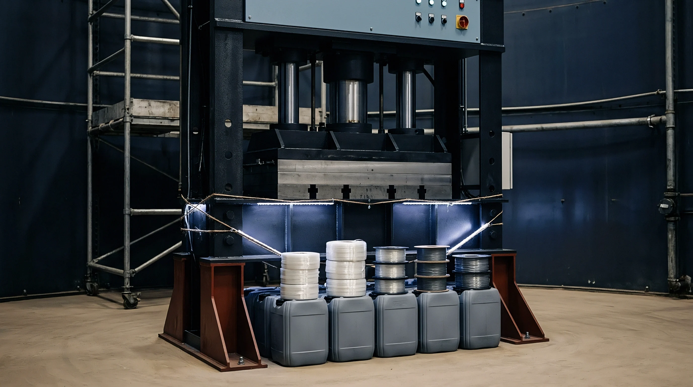
Contract
Procuring raw material test data requires clear specifications to protect tooling investments. When outsourcing characterization, scope-of-work documents should detail exact test conditions rather than requesting generic parameter cards. Defining stretch modes, strain rates, temperatures, pre-conditioning protocols, and optimization routines prevents receiving unusable hyperelastic datasets.
Tooling approval depends heavily on simulation accuracy. A thermoforming die built around faulty thickness predictions can require costly steel recuts, core rebuilds, or plug redesigns. Setting explicit characterization standards in supply contracts assigns financial risk clearly among resin suppliers, testing labs, and toolmakers.
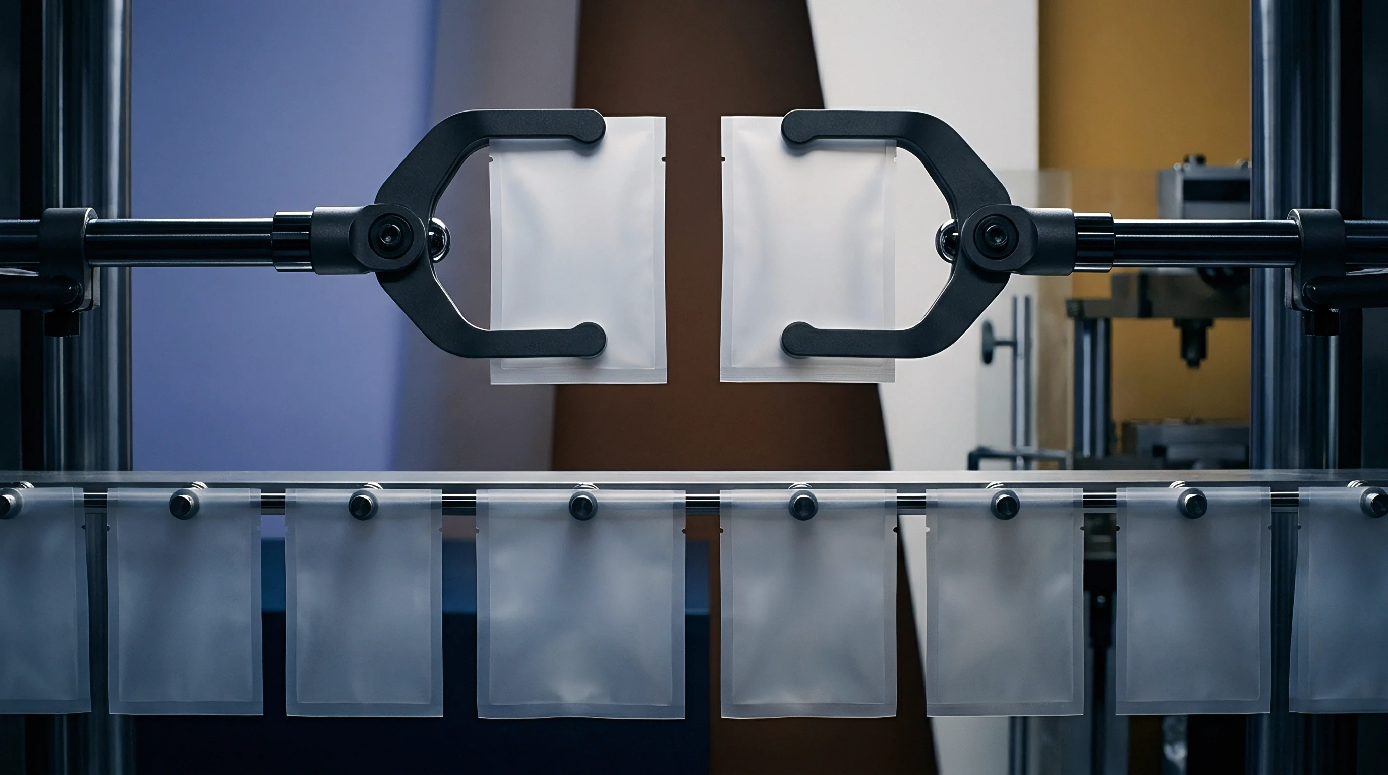
Laboratory Test Dossier Verification
Auditing test dossiers verifies that experimental strain ranges cover actual production forming limits. A complete dossier should include raw force-displacement curves, DIC strain maps, specimen dimensions, and calibration certificates for load cells and optical sensors. Receiving fitted coefficients without the underlying raw curves prevents independent verification.
Verification procedures confirm that regression routines used multi-mode objective functions. The report must list residual errors separately for uniaxial, equal biaxial, and planar modes. Submissions that fail to prove Drucker stability across the expected strain range are rejected before virtual prototyping begins.

Tooling Liability for Simulation Misalignment
When a tool produces out-of-spec parts despite passing FEA checks, financial liability hinges on data provenance. If the simulation relied on single-mode uniaxial parameters provided by a resin supplier, modification costs fall on the procurement team that accepted incomplete data. If a certified lab delivers multi-mode parameters that turn out to be mathematically unstable, rework costs shift to the lab under standard warranty terms.
Contracts should define acceptable error bands between simulated and measured T1 sample wall thicknesses. A common acceptance threshold is plus or minus five percent across critical inspection nodes. Exceeding this tolerance requires the data supplier to re-test the material and re-baseline the simulation at their own expense.

Material Specification Limits for Tool Sign-Off
Establishing parameter tolerance bands ensures production resin lots match design assumptions. Lot-to-lot shifts in molecular weight or filler loading change hyperelastic behavior. Setting acceptable limits on initial shear modulus metrics in raw material contracts keeps sheet inflation behavior consistent across production runs.
Data sheets for elastomers and thermoforming sheet should report validated Ogden parameters alongside standard tensile and elongation metrics. Tool procurement agreements specify multi-axial material cards directly before cutting steel. Requiring transparent constitutive data across the supply chain cuts down on tooling re-works, shortens commissioning cycles, and ensures final part performance.